1 Synchronization
Synchronization is critical to communications system. It helps the system to establish a shared sense of time and frequency between transmitter and receiver. In this section, we will introduce some basic ideas. As we mentioned in all the other sections, we will not plan to list all the algorithms (how could that even be possible?), instead, we will show some basic ideas and wish you will know how to start when you need to deal with a real problem. The code used in this section can be found here.
1.1 Frequency Synchronization
We will use a QPSK signal as an example to show the basic idea of frequency synchronization. The transmitted signal can be written as
where \(f_c\) is the carrier frequency, \(\phi\) is an arbitrary phase (unknown to the receiver side), \(s(t) = s_r(t) + js_i(t)\) is the signal, and \(\Re(.)\) is the operator to take the real part. At the receiver side, the signal is demodulated with carrier (\(f_c^\prime\))1
where the center frequency of the second item is usually much higher than the first item. Thus, it can be easily filtered with a low pass filter, that is, after filtering, only the first item will be left
Don't be scared of the complicated equations above. The procedure is actually straightforward, as shown in Fig. 1.

If \(f_c = f_c^\prime\), such system is called zero IF (intermediate frequency) system. It may suffer from IQ imbalance problem. In particular, since the reference signal \(e^{-j(2\pi f_c^\prime)}\) is complex signal, and usually the analog circuit needs to generate the real and image part, respectively. Any imbalance (e.g., phase, frequency and amplitude) between its real and image parts will distort the signal. To overcome such problem, many application use a non-zero IF. In other words, after demodulation, the signal is centered at a non-zero IF (e.g., \(f_c^\prime = f_c - f_{\textrm{if}}\)).
In this case, the demodulation can be done with the real part of the above reference signal (i.e., \(\cos(2\pi f_c^\prime t)\))
It is easy to see the last two items can be filtered by a low pass filter. Thus, after filtering, only the first two items will be left
You may have noticed the similarity between Eqs. (\ref{eqn:sync_rx_if}) and (\ref{eqn:sync_tx}). What we achieve so far is to down-shift the signal from \(f_c\) to \(f_{\textrm{if}}\).
The procedure is shown in Fig. 2.

As shown in Fig. 3, now it is time to bring the signal to discrete domain, where Eq. (\ref{eqn:sync_rx_if}) is written as
where \(f_s\) is the sampling frequency.

Then, a digital mixer is applied to bring the IF signal to baseband
Again, the center frequency of the second item is much higher than the first item, which can be filtered out easily with an digital low pass filter (Fig. 4). Thus, the baseband signal after low pass filter can be written as

In ideal case, \(\phi=0\) and \(f_{\textrm{if}}^\prime = f_{\textrm{if}}\), where Eq. (\ref{eqn:sync_rx_baseband}) is simplified as
which is same as the transmitted data (Fig. 5).

When the phase error is not zero (i.e., \(\phi\neq 0\)), and frequency error is zero (i.e., \(f_{\textrm{if}}^\prime = f_{\textrm{if}}\)), Eq. (\ref{eqn:sync_rx}) is written as
The constellation is rotated by \(\phi\).

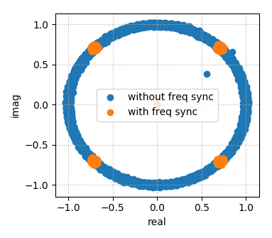
When the frequency offset is not zero, the received constellation will not contain 4 points any more, instead, the received signal can be located anywhere on the unit circle. In Fig. 7, the received constellation looks like 4 clusters. It is because we only show a small amount of data; otherwise, it will be a circle, as the phase error (\(2\pi\frac{f_{\textrm{if}} - f_{\textrm{if}}^\prime}{f_s}+\phi\)) will increase as \(n\) increases.

We have seen the impact of the frequency and/or phase error to the signal constellation. The next question is how to fix it? There are generally two steps
Estimate the phase error. For example, Fig. 8 shows the received and the estimated signals. In some systems, the estimated signal can be the true signal (\(s[n]\), e.g., preamble symbols known at the receiver side). In some systems, it may be from the estimation (e.g., maximum likelihood estimation). Then the phase error is the phase difference between the received and estimated signals
$$ \begin{align} r_b[n]s[n]^{*} &= \left\Vert s[n]\right\Vert^2e^{j\phi_e}\nonumber \\ &= e^{j\phi_e} \end{align} $$where \(s[n]^{*} = s_r[n] - js_i[n]\) is the conjugate of \(s[n]\). Then the phase error can be estimated as
$$ \begin{align} \angle(r_b[n]s[n]^{*}) = \phi_e. \end{align} $$
Fig.8. Phase error estimation. How to calculate the angle/phase? For software simulation (e.g., matlab, scilab, scipy), there is always some function available, which may not be true for real hardware implementation.
Look-up Table. One straightforward way is to use a look-up table, that is, storing the phase corresponding to each point on the unit circle (i.e., \(a+jb\), and \(a^2+ b^2=1\)). Generally we need the phase within range \([-\pi, \pi]\); however, there is no need for the look-up table to cover the whole range, since \(\sin\) and \(\cos\) are symmetric. For example, since
$$ \begin{align} \cos(-\alpha) &= \cos(\alpha),\nonumber\\ \sin(-\alpha) &= -\sin(\alpha), \end{align} $$the look-up table may only store the positive phase. That is, for a complex value \(a+jb\), if \(b\geq 0\), \(\alpha = \alpha_l\), where \(\alpha_l\) is the value in look-up table (indexed with \(a+jb\)); otherwise (\(b<0\)), \(\alpha=-\alpha_l\), where \(\alpha_l\) corresponds to \(a-bj\) in the look-up table. Thus, there is no need to worry about the negative phase (\([-\pi, 0]\)). Furthermore, for phase in \([0, \pi]\), since
$$ \begin{align} \cos(\pi-\alpha) &= -\cos(\alpha),\nonumber\\ \sin(\pi-\alpha) &= \sin(\alpha), \end{align} $$it only needs to store the phase in \([0, \pi/2]\), where the phase in \([\pi/2, \pi]\) can be derived easily. In summary, to look up the phase of \(a+jb\),
- find the phase corresponding to \(|a| + j|b|\), denote it as \(\alpha_l\);
- if \(a\geq 0\) and \(b\geq 0\), the phase is in the first quadrant, i.e., \(\alpha=\alpha_l\);
- if \(a < 0\) and \(b \geq 0\), the phase is in the second quadrant, i.e., \(\alpha=\pi -\alpha_l\);
- if \(a < 0\) and \(b < 0\), the phase is in the third quadrant, i.e., \(\alpha=\alpha_l-\pi\);
- if \(a\geq 0\) and \(b <0\), the phase is in the forth quadrant, i.e., \(\alpha=-\alpha_l\);
It is not bad as we shrink the look up table by a factor of 4 by simple math. Actually if the look up table size is the bottle neck, we can do even better. Considering a phase in \([0, \pi/2]\), we have
$$ \begin{align} \cos(\alpha) &= \sin(\pi/2 - \alpha),\nonumber\\ \sin(\alpha) &= \cos(\pi/2 - \alpha). \end{align} $$It means that the look up table only needs to cover \([0, \pi/4]\). To find the phase of \(a+jb\) in first quadrant (i.e., \(a\geq 0\), \(b\geq 0\)) (the other quadrants can be got as mentioned above)
- calculate \(a_m = \max(a, b)\), and \(b_m = \min(a, b)\);
- find the phase \(\alpha_l\) correspond to \(a_m + jb_m\);
- if \(a_m = a\), then the phase is in \([0, \pi/4]\), i.e., \(\alpha = \alpha_l\);
- if \(a_m = b\), then the phase is in \([\pi/4, \pi/2]\), i.e., \(\alpha = \pi/2 - \alpha_l\).
In practice, the complex value may not be on the unit circle. In this case, before searching the phase in the look-up table, it is helpful to normalized it first
$$ \begin{align} a_n &= \frac{a}{\sqrt{a^2+b^2}},\nonumber\\ b_n &= \frac{b}{\sqrt{a^2+b^2}}. \end{align} $$Apparently, \(\angle(a_n+b_nj)\) is same as \(\angle(a+jb)\), since scaling a complex value wil not change its direction (angle).
Phase Approximation. If the phase error \(\phi_e\) is small,
$$ \begin{align} e^{j\phi_e} &= \cos(\phi_e) + j\sin(\phi_e)\nonumber\\ &\approx 1 + \phi_e. \end{align} $$Thus, the phase error can be estimated by the image part of \(r[n]s[n]^{*}\), that is
$$ \phi_e \approx \Im(r_b[n]s[n]^{*}), $$where \(\Im(.)\) is the operator to take the image part of a complex value.

Fig.9. Phase error estimation when \(\phi_e\) is small. Such assumption may be true once the frequency synchronization converges. Thus, it can be used to simplify the operation. However, it is definitely not true for the initialization period of the frequency synchronization, since the phase offset can be arbitrary. As mentioned above, we need a better approximation in \([0, \pi/4]\).
As described in [1], a phase in \([0,\pi/4]\) can be approximated as
$$ \begin{align} \alpha = \frac{b/a}{1+0.28125(b/a)^2}. \label{eqn:sync_phase_est} \end{align} $$As shown in Fig. 10, the maximum estimation error is roughly 0.28 degree.
>>> alpna = np.linspace(0, np.pi/4, 10000)
>>> a = np.cos(alpha)
>>> b = np.sin(alpha)
>>> alpha_e = (b/a)/(1+0.2815*(b/a)**2)
>>> plt.clf()
>>> plt.plot(alpha*180/np.pi, (alpha-alpha_e)*180/np.pi)
>>> plt.grid('on', ls=':')
>>> plt.xlabel('angle (in degree)')
>>> plt.ylabel('estimation error (in degree)')
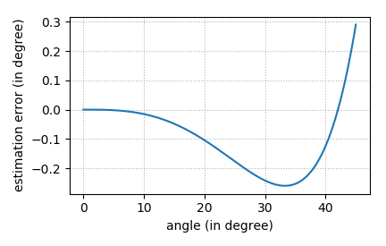
Fig.10. Phase error of the estimation from Eq. (\ref{eqn:sync_phase_est}). CORDIC Algorithm. The CORDIC (COordinate Rotation DIgital Computer) algorithm [2] is an iterative method to estimate the phase. Generally, a phase \(\alpha\) in \([0, \pi/4]\) can be decoupled as
$$ \begin{align} \alpha = \pi/8 + d_1\pi/16 + d_2\pi/32 + \cdots, \end{align} $$where \(d_i = \pm 1\). In other words, if we rotate a complex value by \(\pi/8\) (clockwise), then \(d_1\pi/16\), \(d_2\pi/32\), \(\cdots\), eventually, the phase of the resulting value will approach zero. So one general idea to estimate a phase in \([0, \pi/4]\) could be
- rotate (clockwise) with a phase \(\pi/8\),
- if the resulting value is still in first quadrant, rotate (clockwise) with a phase of \(\pi/16\);
- otherwise, rotate (counterclockwise) with a phase of \(\pi/16\).
- if the resulting value is in first quadrant, rotate (clockwise) with a phase \(\pi/32\),
- otherwise, rotate (counterclockwise) with a phase of \(\pi/32\).
- \(\cdots\)
To rotate a complex value \(a+jb\) by a phase \(\alpha\) (counterclockwise),
$$ \begin{align} a^\prime &= a\cos(\alpha) - b\sin(\alpha),\nonumber\\ b^\prime &= b\cos(\alpha) + a\sin(\alpha). \label{eqn:sync_rotate} \end{align} $$Thus, we can store all the \(\cos(\pi/8)\), \(\sin(\pi/8)\), \(\cos(\pi/16)\), \(\sin(\pi/16)\), \(\cdots\), and follow the above procedure to estimate the phase. However, such procedure is computational complicated, since at each step it needs 4 multiplications and 2 additions. CORDIC algorithm simplifies such procedure. Eq. (\ref{eqn:sync_rotate}) can be written as
$$ \begin{align} a^\prime &= \cos(\alpha)(a - b\tan(\alpha)),\nonumber\\ b^\prime &= \cos(\alpha)(b + a\tan(\alpha)). \label{eqn:sync_rotate2} \end{align} $$If \(\alpha\) is chosen such that \(\tan(\alpha)= d_k 2^{-k}\), where \(d_k\) is the rotation direction, then Eq. (\ref{eqn:sync_rotate2}) can be simplified as
$$ \begin{align} a^\prime &= \cos(\alpha)(a - bd_k 2^{-k}),\nonumber\\ b^\prime &= \cos(\alpha)(b + ad_k 2^{-k}). \label{eqn:sync_rotate3} \end{align} $$Since we only care about the phase and not the amplitude, the phase of \(a^\prime/\cos(\alpha)+jb^\prime/\cos(\alpha)\) is same as \(a^\prime+jb^\prime\). Thus, \(\cos(\alpha)\) can be ignored
$$ \begin{align} a^\prime &= a - bd_k 2^{-k},\nonumber\\ b^\prime &= b + ad_k 2^{-k}. \label{eqn:sync_rotate4} \end{align} $$In this case, Eq. (\ref{eqn:sync_rotate4}) can be easily implemented by shifting and addition. The algorithm is summarized as
$$ \begin{align} a_{k+1} &= a_k- b_k d_k 2^{-k},\nonumber\\ b_{k+1} &= b_k+ a_k d_k 2^{-k},\nonumber\\ \alpha_{k+1} &= \alpha_k - d_k \arctan(2^{-k}), \end{align} $$where
$$ \begin{align} d_k = \begin{cases} 1 & \textrm{if } b_k<0\\ -1 & \textrm{otherwise} \end{cases}. \end{align} $$For the phase in \([0, \pi/4]\), the iteration may look like
def _cordic(a, b, iteration=10):
    """
    return the phase of complex value a+jb

    the phase must be in [0, pi/4]
    """
    alpha = 0
    d = -1
    atan = np.arctan(1./np.power(2., np.arange(1, iteration+1)))
    for k in range(iteration):
        a_n = a - b*d*2**(-k-1)
        b_n = b + a*d*2**(-k-1)
        alpha = alpha - d * atan[k]
        if b_n < 0: d = 1
        else: d = -1
        a, b = a_n, b_n
    return alpha
Then, the arbitrary phase (\([-\pi, \pi]\)) can be got by applying the symmetric properties mentioned above
def cordic(a, b, iteration=10):
    """
    return the phase of complex value a+jb

    return the phase (-pi, pi]
    """
    a_m = np.max((np.abs(a), np.abs(b)))
    b_m = np.min((np.abs(a), np.abs(b)))
    alpha = _cordic(a_m, b_m, iteration)
    if a_m != np.abs(a):
        alpha = np.pi/2-alpha
    if a < 0 and b >= 0:
        alpha = np.pi - alpha
    elif a < 0 and b < 0:
        alpha = alpha - np.pi
    elif a >= 0 and b < 0:
        alpha = -alpha
    return alpha
Fig. 11 shows the maximum estimation errors from the CORDIC algorithm. The error is smaller with more iterations, as expected.
>>> alpha = np.linspace(-np.pi, np.pi, 10000)
>>> alpha_err = np.zeros(10)
>>> for iteration in range(5, 15):
...     t = np.zeros_like(alpha)
...     for i, p in enumerate(alpha):
...         t[i] = cordic(np.cos(p), np.sin(p), iteration)
...     alpha_err[iteration - 5] = np.max(np.abs(t-alpha))
>>> plt.clf()
>>> plt.plot(np.arange(5, 15), alpha_err*180/np.pi, '-o')
>>> plt.xlabel('iterations')
>>> plt.ylabel('max estimation error (in degree)')
>>> plt.grid('on', ls=':')

Fig.11. Maximum estimation error of the CORDIC algorithm. Compensate Phase Error. The estimated error is used to adjust the system such that the phase error is decreased. For example, the phase error will be sent to a PI (proportional and integral) controller (Fig. 12)
$$ \begin{align} e[n] &= e_p[n] + e_i[n], \end{align} $$where
$$ \begin{align} e_p[n] &= g_p\phi_e[n]\nonumber\\ e_i[n] &= e_i[n-1] + g_i\phi_e[n]. \end{align} $$
Fig.12. Structure of a PI controller. For example, as shown in Fig. 13, \(e[n]\) is sent to the block that generates \(f_c^\prime\) or to the block that generates \(f_{\textrm{if}}^\prime\)2. In our example, frequency down-shifting with \(f_c^\prime\) is done in analog domain. Thus, \(e[n]\) needs to send to a DAC block to generate the analog signal (e.g., \(e(t)\)) before sending to \(f_c^\prime\). Such process brings more cost. However, it makes sure that the analog LPF block works in ideal condition when the frequency synchronization converges. Otherwise, if \(f_{\textrm{if}}\) is too far away from \(f_{\textrm{if}}^\prime\), the signal band may not be in the passband of the analog low pass filter, which causes distortion to the signal.

Fig.13. Structure of phase error compensation. On the other side, compensating \(e[n]\) at \(f_{if}^\prime\) is much easier, since both the error signal \(e[n]\) and the NCO (numerically controlled oscillator) are in digital domain. The NCO block generates the reference signal for frequency down-shifting to get the baseband signal (by multiplying \(e^{j\phi_{\textrm{nco}}}\)), where
$$ \begin{align} \phi_{\textrm{nco}}[n] = \phi_{\textrm{nco}}[n-1] - 2\pi\frac{f_{\textrm{if}}^\prime}{f_s} - e[n]. \end{align} $$In Fig. 13, the phase error (\(e[n]\)) is sent to the NCO for frequency synchronization. Thus, there is a delay (\(D\)) between phase error estimation and compensation (e.g., the delay from the digital LPF). If the delay is large, it may limit the maximal frequency offset the system can deal with. For example, at time \(n\), the estimated phase error is positive, while at time \(n+D\), the phase error may be negative due some large frequency offset. If we use \(e[n]\) to compensate for the phase error of sample \(n+D\), the system may diverge. Thus, in some system, to minimize the delay \(D\), we may put a phase rotation block right before the decision block (Fig. 14).

Fig.14. Structure of phase error compensation to minimize the delay \(D\).
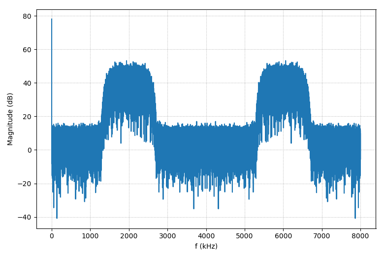
In the following example, we will show how to do the frequency synchronization for a QPSK signal (Fig. 5). First, let us define some parameters. The signal bandwidth is 1 MHz (centered at 2 MHz IF) with sampling rate 8 MHz.
>>> # parameters
>>> Fsym = 1e6 # symbol rate
>>> UPS = 8 # up-sampling factor
>>> Fif = 2e6 # IF frequency
>>> # IF frequency delta at receiver side with frequency error
>>> Fif_prime = Fif + 20e3
>>> Fif_phi = 0.1
>>> Fs = Fsym*UPS # sampling frequency
>>> SNR = 30 # awgn (dB)
>>> # Modulation
>>> MODE = 4
>>> PHASE_OFFSET = np.pi/MODE
>>> # the maximum phase error without bit error
>>> PHASE_SPACE = 2*np.pi/MODE/2
>>> #mapping table for hard decision
>>> PHASE = 2*np.pi/8*np.array([1, 3, -3, -1])
>>> # True --> hard decision; False --> use tx data
>>> DECISION = False
Generate the random QPSK symbols at 1 MHz, which are up-sampled to 8 MHz by inserting zero. Then, the result signal is low-pass filtered to suppress mirrors.
>>> # generate the PSK signal
>>> symbol = np.floor(MODE*np.random.rand(10000))
>>> signal = np.exp(1j*(2*np.pi/MODE*symbol + PHASE_OFFSET))
>>> # tx shaping filter
>>> fir_tx = rcosdesign(0.4, 5, UPS)
>>> s = np.kron(signal, np.concatenate((np.ones([1]), np.zeros([UPS-1]))))
>>> s = scipy.signal.lfilter(fir_tx, 1, s)
>>> # remove the filter delay
>>> s = s[(len(fir_tx)-1)//2:]
Up-shift the baseband signal to IF to simulate a received signal after ADC.
>>> # rx
>>> # modulation with IF to simulate a received signal after ADC
>>> r = np.real(s*np.exp(1j*2*np.pi*Fif/Fs*np.arange(len(s)))+Fif_phi)
>>> # add AWGN
>>> noise = np.random.normal(0, 1, len(r))
>>> noise *= 10**(-SNR/20)*np.sqrt(np.mean(r*r))*np.sqrt(UPS)
>>> r += noise
Before we start the frequency synchronization loop, let us define some variables.
>>> # match filter
>>> fir_rx = rcosdesign(0.4, 3, UPS)
>>> r_buf = np.zeros(len(fir_rx), dtype=complex)
>>> # frequency synchronization
>>> q = np.zeros(np.ceil(len(s)/float(UPS)).astype(int), dtype=complex)
>>> q_est = np.zeros(np.ceil(len(s)/float(UPS)).astype(int), dtype=complex)
>>> freq_est = np.zeros(np.ceil(len(q)).astype(int))
>>> # estimated error
>>> ph_nco = 2*np.pi*(Fif_prime)/Fs
>>> freq_err = 0.0
>>> freq_err_i = 0.0
>>> freq_err_d = 0.0
fir_rx is the coefficients for the low pass filter after down shifting (\(f_{\textrm{if}}^\prime\)). Now we can do the actual frequency recovery loop.
>>> index = 0
>>> # down sampling by a factor of UPS, then estimate the frequency error,
>>> # assume no clock error and sampling at best phase
>>> for i in range(0, len(r)):
...     # step 1: NCO for frequency synchronization & frequency error compensation
...     ph_nco = ph_nco - freq_err - 2*np.pi*(Fif_prime)/Fs
...     if ph_nco > np.pi:
...         ph_nco -= 2*np.pi
...     elif ph_nco < -np.pi:
...         ph_nco += 2*np.pi
...     # step 2: down shift
...     r_b = 2*r[i]*np.exp(1j*ph_nco)
...     # step 3: filtering
...     r_buf = np.roll(r_buf, 1)
...     r_buf[0] = r_b
...     r_b = np.sum(r_buf*fir_rx)
...     # step 4: down-sampling by a factor of 8
...     if i >= (len(fir_rx)-1)/2 and i%UPS == 0:
...         # step 5: received signal
...         z_in = r_b
...         q_est[index] = z_in
...         # step 6: decision
...         if DECISION == 0:
...             q_h = signal[index]
...         else:
...             # find the closest point on constellation
...             p = np.arctan2(q_est[index].imag, q_est[index].real)
...             b = np.argmin(np.abs(p-PHASE))
...             q_h = np.exp(1j*PHASE[b])
...         # step 7: estimate frequency error
...         # remove the signal phase
...         q[index] = q_est[index]*np.conj(q_h)
...         # phase error ~ [-pi, pi]
...         phi_e = np.arctan2(q[index].imag, q[index].real)
...         # step 8: PI controller
...         freq_err_i = freq_err_i + phi_e*0.01/UPS
...         freq_err_d = phi_e*0.2/UPS
...         freq_err = freq_err_i + freq_err_d
...         freq_est[index] = freq_err
...         index += 1
As shown in the above code
- Step 1. Calculate the phase for down-shifting the IF signal to baseband. The phase includes two items: one from \(f_{\textrm{if}}^\prime\), and the other from the estimated phase error. It is a good idea to limit the phase in \([-\pi, \pi]\). Otherwise, when the phase becomes very big, the round error from float/double value will be unacceptable.
- Step 3. For simplicity, the LPF is done with naive implementation. You should never do this for real.
- Step 4. For simplicity, we assume the system does not have clock error (i.e., the transmitter and receives have the exact same clock rate, which is not true in practice.). And we also manually find the best sampling phase, which should be recovered by the clock synchronization in real.
Step 6. There are generally two ways to get the hard value of the received signal. In some systems (e.g., 802.11a), the system may send some preamble, which is known at the receiver side. In this case, the hard value is the true value of the transmitted preamble signal. In some systems, such preamble is not available (e.g., too expensive). In this case, the point on the constellation that is closest to the received signal may be viewed as the hard value. Such method has some obvious drawbacks. For example, as shown in Fig. 17, since the system has a large phase error \(\phi_e\), the point on the constellation that is closest to the received signal is the orange point, instead of the blue point. Then, the estimated error will be \(\hat{\phi}_e\), rather than \(\phi_e\).

Fig.17. Illustration of large phase error.
Figs. 18 and 19 show the simulation result. With 20 kHz frequency offset, the signals without frequency synchronization show as a blue circle on the constellation, as expected; while after frequency synchronization, the signals converges to a QPSK constellation.
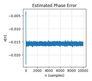
And the estimated phase error \(e[n]\) converges to a constant which is close to \(-2\pi\frac{20e3}{8e6} = -0.0157\).
1.2 Clock Synchronization
The main purpose of clock synchronization (or clock/timing recovery, symbol synchronization) is to find the optimal sampling phase and rate. Let's start with the simplest BPSK case. For example, Fig. 20 shows 2 possible sampling phases. It is obvious that the sampling phase indicated by the blue dash line is better than the red one, where the signal is stronger, suffers less from ISI and is more robust to random noise.

For BPSK signal, one way to achieve clock synchronization is to check the time when the signal crosses zero. The zero-crossing position may correspond to a sample which is either zero (i.e., \(r[n]=0\)), or changes sign/phase from its previous sample (i.e., \(r[n]r[n-1]<0\)). For example, as shown in Fig. 21, the blue dash line shows the optimal sampling phase, and the up-sampling rate is 24. Then the optimal sampling timing will be roughly 12 samples (0.5 symbols) from any zero crossing position (indicated by the red dots). So one straightforward algorithm is to check the distance between the last sampling position and adjacent zero crossing point. If the distance is not 12 samples (0.5 symbols), update the next sampling phase accordingly.

It is easy to see such algorithm suffers from long run 1 or -1. The red dots in Fig. 22 shows the expected zero-crossing positions, which are apparently not close to zero since there is no phase change between adjacent symbols. In this case, the algorithm won't be able to update the sampling phase during that long run 1 or -1 period. In practice, such long run 1 or -1 should be avoided, for example, by the scramble block in the transmitter or modulation schemes (e.g., bi-phase).

The zero-crossing algorithm works well for 'clean' signal. However, if the signal suffers from noise, the zero-crossing position will not occur once between two adjacent symbols (with phase change). Instead, it may occur multiple times within a symbol, or the cross-zero position will not be one sample, but a region. Thus, it will be difficult to determine the phase error.
Another widely used algorithm is called early-late gate method. For each symbol, we will get three samples (Fig. 23)
- one at the estimated optimal sampling time (\(r_{on}\));
- one before the estimated optimal sampling time (\(r_{early}\));
- one after the estimated optimal sampling time (\(r_{late}\)).
Don't be confused. Here the estimated optimal sampling time may be far away from the optimal sampling time. Usually, the distance between samples \(r_{on}\) and \(r_{early}\) is chosen to be same as the one between \(r_{on}\) and \(r_{late}\). The algorithm adjusts the sampling phase dynamically by comparing these three samples. The goal of the clock synchronization is to minimize \(|r_{late}-r_{early}|\) (Fig. 23).

Sampling too early. Fig. 24 shows the early sampling case, where the estimated sampling phase is before the optimal one. In this special case, \(r_{late}\) is larger than \(r_{early}\), which can be used to adjust the sampling phase of the next samples (e.g., delay the sampling time).

Sampling too late. Similarly, Fig. 25 shows the late sampling case, where \(r_{late}\) is smaller than \(r_{early}\). Thus, the next samples need to be sampled early.

We will use an example with BPSK signal to show how to achieve clock synchronization with the early-late gate method3. As usual, we first define some parameters used in the simulation. The data/symbol rate is very small (~1 kHz), thus the sampling rate can be relatively high (e.g., 128 times of the data/symbol rate).
>>> # parameters
>>> Fs = 152000 # sample frequency(Hz)
>>> Fd = 1187.5 # data rate(Hz)
>>> CLK_OFFSET = 200e-6 # (+/-200ppm)
>>> SNR = 7 # in dB
We prepend a PN (pseudo-noise) sequence in front of the message bits, so that at the receiver side we can easily find the start of the message bits with a correlation to calculate the BER (bit error rate). The 127 bits PN sequence is generated with an LFSR (linear-feedback shift register). We also append some zeros at the end of the message bits, just to push all the data bits through the filters.
>>> msg_bits = np.random.randint(0, 2, 1000)
>>> # add PN sequence for frame synchronization
>>> pn = sync_lfsr()
>>> msg_cyc = np.hstack((pn, msg_bits, np.zeros(5, dtype=int)))
Then, we add a differential encoding, such that the system can tolerate 180 phase ambiguity (e.g., as mentioned in the frequency synchronization section).
>>> # differential encoding
>>> bit_p = 0
>>> for i in range(len(msg_cyc)):
...     msg_cyc[i] = np.bitwise_xor(bit_p, msg_cyc[i])
...     bit_p = msg_cyc[i]
Its encoding and decoding schemes are shown in Tables. 1 and 2, respectively.
| Prev output | Current input | Current output |
|---|---|---|
| 0 | 0 | 0 |
| 0 | 1 | 1 |
| 1 | 0 | 1 |
| 1 | 1 | 0 |
The potential drawback of differential coding is the 'error propagation'. As shown in Table. 2, the current decoding output relies on both the current input and the previous input. If the previous input is wrong, the decoding output may be wrong too.
| Prev input | Current input | Current output |
|---|---|---|
| 0 | 0 | 0 |
| 0 | 1 | 1 |
| 1 | 0 | 1 |
| 1 | 1 | 0 |
The next step is shaping filter, which is defined as
where \(t_d = \frac{1}{f_d}\). Its frequency and impulse responses are shown in Fig. 26.

To generate the filter coefficients, we first build the filter in frequency domain, then convert it to time domain with IFFT.
>>> # BPSK modulation
>>> # in real case this may be replaced by a lookup table, rather than a filter
>>> # generate the shaping filter
>>> UP_SAMP = int(Fs/Fd)
>>> UP_BASE = UP_SAMP//2
>>> hf = np.zeros(np.ceil(UP_SAMP/2*UP_BASE/2).astype(int))
>>> hf[:UP_BASE] = np.cos(np.pi/4*np.linspace(0, 2, UP_BASE))
>>> hf = np.hstack((hf, hf[-1:0:-1]))
>>> ht = np.fft.ifft(hf)
>>> ht = np.hstack((ht[-1 - (len(ht)-1)//2-1-1:], ht[0:(len(ht)-1)//2]))
>>> # hard coded here, 401 taps around center, just for simulation
>>> ht = ht[2048-200:2048+201].real
Before applying the shaping filter, the signal bits are up-sampled by a factor of 2. In particular, 1 and 0 is replaced with \([1, -1]\) and \([-1, 1]\), respectively. The waveforms after shaping filter are shown in Fig. 27. It is easy to see that there is always a zero-crossing within each symbol. Such fact can be used for clock synchronization with the zero-crossing method mentioned above.

>>> # generate bi-phase symbol
>>> msg_biphase = np.kron(msg_cyc*2-1, [1, -1])
>>> # shaping filter
>>> u = np.zeros(UP_BASE)
>>> u[0] = 1
>>> msg_shaping = scipy.signal.lfilter(ht, 1, np.kron(msg_biphase, u))*UP_BASE
Now it's time to add clock error and noise.
>>> # add clock error
>>> msg_signal = rx_src(msg_shaping, Fs, Fs*(1+CLK_OFFSET))
>>> # add noise
>>> gain = 1.0/(np.sum(msg_signal*msg_signal)/len(msg_signal))/(Fs/Fd/4)
>>> msg_signal = np.sqrt(gain)*msg_signal
>>> noise = np.random.normal(0, 1, len(msg_signal))
>>> noise *= 10**(-SNR/20)*np.sqrt(np.mean(msg_signal*msg_signal))*np.sqrt(UP_BASE)
>>> msg_signal += noise
The clock error is added with function rx_src. When implementing rx_src, we need to make sure it works as intended.To do that, we can use a sinusoid signal for testing. For example, the following code adds 100 ppm offset to the sampling frequency (e.g., 24 MHz) of a sinusoid signal (e.g., 1 MHz). Since the signal length is 10000, the result signal will have roughly 1 (10000*100e-6) additional sample. As shown in Fig. 28, at the beginning \(n\approx 0\), two signals matched with each other very well; while \(n\approx 10000\), compared to the original signal, (s) the result signal (s2) is roughly 'delayed' by 1 sample. In other words, within a period of roughly 10000 samples, s2 has one more samples than s, as expected.
>>> s = np.cos(2*np.pi*1e6/24e6*np.arange(10000))
>>> s2 = rx_src(s, 24e6, 24e6*(1+100e-6))

Another test we can do is to apply the rx_srcs twice to get the signal at the original frequency. The result should be as close to the original signal as possible.
>>> s3 = rx_src(s2, 24e6*(1+100e-6), 24e6)
>>> np.mean(np.abs(s[100:len(s3)]-s3[100:]))
2.3175959195405037e-05
The received signal is then down-sampled by a factor of 8, so the clock synchronization is done at sampling rate of \(152/8=19\) kHz (or 16 times of the symbol rate). Such choice is kind of 'arbitrary', and should base on the application. Generally, the higher the sampling rate, the better the clock synchronization performance.
>>> # BSKP demodulation
>>> # down sampling by factor 8
>>> rx_sig = msg_signal
>>> fir_ds8 = scipy.signal.firwin2(40, [0, 4750./(Fs), 14250./(Fs), 1], [1, 1, 0, 0])
>>> rx_sig = scipy.signal.lfilter(fir_ds8, 1, rx_sig)
>>> rx_sig = rx_sig[::8]
The down-sampled signal is then sent to a matching filter, which has the same shape as the waveform shown in Fig. 27 (except the sampling rate).
>>> # generate the matching filter
>>> hf8 = np.zeros(int(UP_SAMP/8/2*UP_BASE/2))
>>> hf8[:UP_BASE] = np.cos(np.pi/4*np.linspace(0, 2, UP_BASE))
>>> hf8 = np.hstack((hf8, hf8[-1:0:-1]))
>>> ht8 = np.fft.ifft(hf8)
>>> ht8 = np.hstack((ht8[-1- (len(ht8)-1)//2-1-1:-1], ht8[:(len(ht8)-1)//2]))
>>> # filter the signal from bit '1'
>>> s = np.hstack((np.ones(8), -1*np.ones(8), np.zeros(len(ht8))))
>>> fir_match = scipy.signal.lfilter(ht8, 1, s)
>>> fir_match = fir_match[246:285].real
>>> # match filtering
>>> rx_sig = scipy.signal.lfilter(fir_match, 1, rx_sig)
Now it is time for clock synchronization and BPSK demodulation
>>> # Timing recovery and BPSK demodulation
>>> rx_bits, smp_time = sync_clk_bpsk(rx_sig, UP_SAMP/8, 1)
Function sync_clk_bpsk implements the early-late gate method for clock synchronization. For each symbol, three samples are compared to adjust the sampling phase of the next symbol. For simplicity, in the demo, we directly apply the estimated error to the sampling phase. In some application, it may be helpful to send the estimated error to a PI controller first. The implementation find the 'best' phase in all the 16 possible phases. In other words, the performance is only 'optimal' within these 16 phases. If the optimal phase is beyond these 16 phases, there is no way to find the optimal one. Thus, the higher the sampling rate, the better the performance. In the next example, we will show how to use interpolation to approach the optimal sampling phase without requiring a high sampling frequency. For this demo, 16 phases is enough to get a good result.
Here, the 'early' and 'late' samples are the neighbours of the 'on' sample, that is the distance between the 'early' (or 'late') sample and the 'on' sample is 1 sample. You may try different values to compare the performance4.
def sync_clk_bpsk(signal, ups, dis=1):
    PERIOD = ups  # upsample factor
    sample_ins = dis + 8 #initial sample position
    # output
    smp_tm = np.zeros(np.ceil(len(signal)/float(PERIOD)).astype(int)+1)
    msg = np.zeros(np.ceil(len(signal)/float(PERIOD)).astype(int)+1)

    ds_cnt = 0 # down-sampling counter
    sym_cnt = 0 # current symbol index after down-sampling
    for i in range(int(np.floor((len(signal)))-dis)):
        ds_cnt += 1
        if ds_cnt >= sample_ins:
            ds_cnt = 0
            s_early, s_on, s_late = signal[[i-dis, i, i+dis]]
            if (s_on - s_early)*(s_on - s_late) > 0:
                # on time sampling
                sample_ins = PERIOD
            elif s_on*(s_on - s_early) > 0 and s_on*(s_on - s_late) < 0:
                # early sampling, delay the next one
                sample_ins = PERIOD + 1
            elif s_on*(s_on - s_early) < 0 and s_on*(s_on - s_late) > 0:
                # late sampling, advance the next one
                sample_ins = PERIOD - 1
            smp_tm[sym_cnt] = i
            # decision slicer
            msg[sym_cnt] = signal[i] > 0
            sym_cnt += 1
    return (msg.astype(int), smp_tm.astype(int))
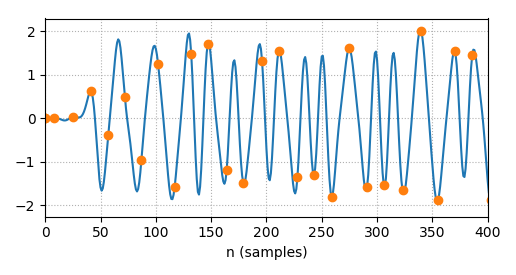
Fig. 29 shows the signal after matched filter and the estimated sampling time (indicated by the orange dots). After several symbols, the sampling phases are converged to the peaks or valleys, which means the clock synchronization algorithm works well.
After that, it is trivial to find the frame head with a correlation, so that we can calculate the BER. With the setup shown above, you should see zero bit error.
>>> # differential decoding
>>> rx_bits_diff = np.bitwise_xor(np.hstack(([0], rx_bits[:-1])), rx_bits)
>>> # frame synchronization
>>> sync_corr = scipy.signal.convolve(rx_bits_diff*2-1, np.flipud(pn)*2-1)
>>> start = np.where(sync_corr > 80)[0]
>>> if len(start) == 0:
...     print('Frame Header error!')
>>> else:
...     print('Frame Header: %d at %d'%(sync_corr[start[0]], start[0]))
...     msg_rx = rx_bits_diff[start[0]+1:]
...     lenmin = min(len(msg_bits), len(msg_rx))
...     err = sum(abs(msg_bits[:lenmin] - msg_rx[:lenmin]))
...     print('BER: %f (%d/%d)'%(float(err)/lenmin, err, lenmin))
The methods discussed above require multiple samples per symbol. Thus, it is suitable for the low symbol rate system; while for the high symbol rate system, the required sampling rate may be too large to be feasible. Fortunately, there are algorithms that can work on symbols directly. One famous timing recovery algorithm is Mueller-Muller algorithm [3]. For example, Fig. 30 shows the sampling phase and ISI of a system, where \(f\) is the total channel response (e.g., from the shaping filter). Apparently, the sampling phase is delayed by \(\tau\) from the optimal sampling. It causes ISI to the previous symbol (e.g., \(\propto f(\tau-1)]\)), and to the next symbol (e.g., \(\propto f(\tau+1)\)). MM method tries to minimize \(|f(\tau-1)-f(\tau+1)|\).

The phase error can be written as [3]
where \(r[n]\) is the received signal, i.e.,
\(\bar{r}[n]\) is the corresponding true value. Then
The second equation comes from the fact that \(\bar{r}[l]\) and \(\bar{r}[m]\) (\(l \neq m\)) are uncorrelated (i.e., \(E(\bar{r}[l]\bar{r}[m])=0\)). If \(\bar{r}[n]^2\) is constant (e.g., 1), then
It is easy to understand the algorithm with examples. Here we assume everything is ideal, except the sampling clock (e.g., phase, rate):
Optimal sampling. Fig. 31 shows the ideal case. We sample the data at \(n=\cdots, -1, 0, 1, \cdots\), where the ISI is zero. The estimated error with MM algorithm is also zero

Sampling too late. As shown in Fig. 32, the sampling interval is same as the previous case. However, the sampling phase is offset by 0.25 symbol period from the optimal case. The estimated error is

Sampling too early. As shown in Fig. 33, the sampling interval is same as the previous case. However, the sampling phase is offset by 0.25 symbol period to the left from the optimal case. The estimated error is

Sampling too fast. As shown in Fig. 34, the sampling interval is smaller than the optimal case. When the previous sample is sampled at optimal phase, the current sample is sampled too early. In this case,

Sampling too slow. As shown in Fig. 35, the sampling interval is same as the previous case. However, the sampling phase is offset by 0.25 symbol period to the left from the optimal case. In this case,

In the above examples, the signal is assumed to be real. For complex signal (i.e., \(r[n]=r_r[n]+r_i[n]\)), the timing error can be estimated as \(e[n] = e_r[n] + e_i[n]\), where
It is equivalent to
Same as the frequency synchronization case, the estimated error is sent to a PI controller before compensation (Fig. 12). The next question is how to compensate the estimated timing error? For example, Fig. 36 shows that the we need a sample at time \(\tau\) (indicated by a red line), but the previous block only gives us sample at time \(\cdots, -2, -1, 0, 1, 2, \cdots\).

One obvious solution is to apply the timing error to the previous block, such that it changes its sampling phase and output the sample at the right phase. For example, we may delay the sampling phase of a ADC block by \(\tau\).
Another solution is to use interpolation with the existing samples. For example, if \(\tau\) is a rational number (e.g., 1/4), then as mentioned in the Sampling Rate Conversion section, the sample at \(\tau\) can be got by
- up-sampling the system by a factor of 4;
- low pass filtering;
- retrieve the sample at time \(\tau\) (equivalent to align the center filter coefficient (e.g. \(f(0)\)) at time \(\tau\) as shown in Fig. 37).
The procedure is illustrated in Fig. 37, that is
where \(f\) is the filter coefficients, \(k\) is integer. As shown in Sampling Rate Conversion section, if the up-sampling factor (e.g., 4) is known in advance, we can design a filter at 4 times the sampling rate, such that \(f(-1/4+k)\) is available. However, for timing synchronization case, \(\tau\) may be arbitrary. And even if it is a rational number, its corresponding denominator may be too large to pre-design a filter. In this case, it is preferred to design a sampling rate conversion filter at a reasonably high sampling rate, then use interpolation to estimate the filter coefficient if there is no one for a certain phase.

Now we have all the blocks for clock synchronization, its structure may look like

In the following example, we will show how to do the clock synchronization for a QPSK signal (Fig. 5). The signal bandwidth is 1 MHz (centered at 2 MHz IF) with sampling rate 8 MHz. In this demo, we assume the sampling clock at the receiver side is not exactly same as the transmitter (e.g., with 100 ppm offset).
>>> Fsym = 1e6 # symbol rate
>>> UPS = 8 # up sampling factor
>>> Fs = Fsym*UPS # tx sampling rate
>>> Fs_rx = Fs*(1+100e-6) # rx sampling rate with clock offset
>>> DECISION = False # True --> hard decision, False --> use true signal
>>> SNR = 30 # awgn (dB)
>>> # Modulation
>>> MODE = 4
>>> PHASE_OFFSET = np.pi/MODE
>>> # the maximum phase error without bit error
>>> PHASE_SPACE = 2*np.pi/MODE/2
>>> #mapping table for hard decision
>>> PHASE = 2*np.pi/8*np.array([1, 3, -3, -1])
The QPSK signal at 1 MHz is up-sampled by a factor of 8 (insert 0).
>>> symbol = np.floor(MODE*np.random.rand(10000))
>>> signal = np.exp(1j*(2*np.pi/MODE*symbol + PHASE_OFFSET))
>>> # tx shaping filter
>>> fir_tx = rcosdesign(0.4, 3, UPS)
>>> s = np.kron(signal, np.concatenate((np.ones([1]), np.zeros([UPS-1]))))
>>> s = scipy.signal.lfilter(fir_tx, 1, s)
>>> # remove the filter delay
>>> s = s[(len(fir_tx)-1)//2:]
At the receiver side, the signal is sampled with clock Fs_rx, which is achieved by function rx_src.
>>> # rx
>>> # add timing error
>>> r = rx_src(s, Fs, Fs_rx)
>>> # add AWGN
>>> noise = np.random.normal(0, 0.5, len(r)*2)
>>> noise = noise[::2] + 1j*noise[1::2]
>>> noise *= 10**(-SNR/20)*np.sqrt(np.mean(r*np.conj(r)).real)*np.sqrt(UPS)
>>> r += noise
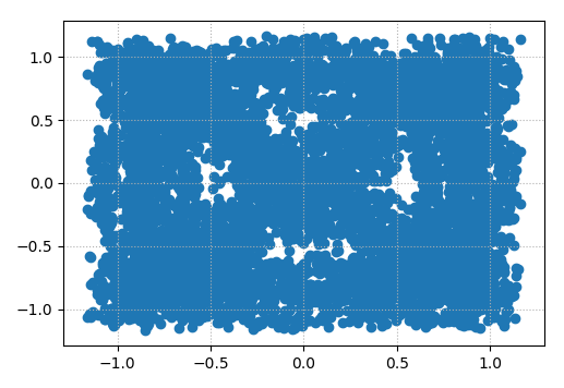
If we down-sample the received signal without clock synchronization, the signal will look like the one shown in Fig. 39. It is even very difficult to tell the signal is from a QPSK constellation.
Then the received signal is filtered with the matched filter. For simplicity, in this demo, we apply the clock synchronization after the matched filter. The risk is if the offset between the transmitter and receiver clocks is large, it will cause ISI even if the offset is compensated later perfectly, since the matched filter is not working in ideal case. Thus, in some application, the clock offset may be compensated before the matched filter; however, in this case, it will introduce more delay between the timing error estimation and compensation.
>>> # match filter
>>> fir_rx = rcosdesign(0.4, 3, UPS)
>>> z = scipy.signal.lfilter(fir_rx, 1, r)
>>> # remove the filter delay
>>> z = z[(len(fir_rx)-1)//2:]
The last thing before we run the clock synchronization loop is to define some variables. In this demo, we estimate the timing error at symbol rate (1 MHz), and the error is compensated at sampling rate (\(\approx\) 8 MHz). Thus, the poly-phase filter is run at sampling rate, while its coefficients is designed at 20 times the sampling rate.
>>> # estimated error
>>> timing_err = 0.0
>>> timing_err_p = 0.0
>>> timing_err_i = 0.0
>>> # hard & soft values and phase error of previous symbol
>>> z_h_p, z_s_p, ph_e_p = 0, 0, 0
>>> # index & counter for down-sampling by a factor of UPS
>>> ds_idx, ds_cnt = 0, UPS-1
>>> # timing recovery parameters
>>> ORDER = 16 #the filter order in Fs sampling rate
>>> M = 20 # up sampling factor
>>> N = M # down sampling factor
>>> flt = scipy.signal.firwin2(ORDER*M+1, [0, 0.5/M, 1.0/M, 1], [1, 1, 0, 0])
>>> # only saving the right half coefficients
>>> flt = flt[ORDER*M//2:]
>>> flt = np.hstack((flt, np.zeros(M+1)))
>>> # timing recovery block initialize value
>>> alpha = 2*M
>>> z_buf = np.zeros(ORDER+1, dtype=z.dtype)
>>> for i in range(ORDER//2):
...     z_buf[ORDER//2-1-i] = z[i]
Now we have everything to run the clock synchronization loop. As shown in Fig. 38, it generally has two components: timing error compensation and estimation.
The timing error compensation is done with an SRC (sampling rate conversion) block, as shown in the first while loop. The code is familiar to us, except the section to generate the coefficients. Besides a fixed step, the sampling phase is also dynamically adjusted by the estimation error (timing_err). Since the poly-phase filter is designed at 20 times of the sampling rate at the receiver side, there are 20 phases available. However, the estimated timing error may align the filter arbitrary with the input samples. In some cases, the filter phase may not be available for filtering. In such case, linear interpolation is applied to estimate the filter coefficient (for example, phase 10.2 may be estimated with phase 10 and 11 with linear interpolation).
The timing error estimation is done in the second while loop. It basically down-samples the output from the previous SRC loop by a factor of 8 to get the symbol, then estimates the error with MM algorithm. The error is filtered with a PI controller before sent to the previous SRC loop.
>>> for i in range(ORDER//2, len(z)):
...     # shift in one data for timing recovery
...     z_buf = np.roll(z_buf, 1)
...     z_buf[0] = z[i]
...     # update the alpha
...     alpha -= M
...     # timing recovery
...     while alpha <= M:
...         output = 0
...         # left side
...         delta = M - alpha
...         for k in range(ORDER//2+1):
...             delta_i = int(delta+k*M)
...             delta_f = delta+k*M - delta_i
...             coeff_k = flt[delta_i]*(1-delta_f) + flt[delta_i+1]*delta_f
...             output += coeff_k*z_buf[ORDER//2-k]
...         # right side
...         delta2 = M-delta
...         for k in range(ORDER//2):
...             delta_i = int(delta2+k*M)
...             delta_f = delta2+k*M - delta_i
...             coeff_k = flt[delta_i]*(1-delta_f) + flt[delta_i+1]*delta_f
...             output += coeff_k*z_buf[ORDER//2+1+k]
...         #output
...         z2[idx_tr] = output*M
...         idx_tr += 1
...         # next output position
...         alpha += N
...         # compensate the timing error
...         alpha += timing_err
...     # down sampling by factor UPS, calculate the timing error,
...     while idx_tr_p < idx_tr:
...         # new input from the sampling rate conversion block
...         z_in = z2[idx_tr_p]
...         idx_tr_p += 1
...         ds_cnt += 1
...         # sampling for hard decision and timing error estimation
...         if ds_cnt >= UPS:
...             ds_cnt -= UPS
...             # hard decision
...             if DECISION == 0:
...                 z_h = signal[ds_idx]
...             else:
...                 ph = np.arctan2(z_in.imag, z_in.real)
...                 b = np.argmin(np.abs(ph-PHASE))
...                 z_h = np.exp(1j*PHASE[b])
...             # timing error calculating
...             e_c = z_in*np.conj(z_h)
...             ph_e = np.arctan2(e_c.imag, e_c.real)
...             # calibrate
...             if abs(ph_e_p) > PHASE_SPACE or abs(ph_e) > PHASE_SPACE:
...                 tmer = 0
...             else:
...                 tmerr = np.real(np.conj(z_h_p)*z_in - np.conj(z_h)*z_s_p)
...             # for next symbol
...             z_s_p, z_h_p, ph_e_p = z_in, z_h, ph_e
...             # PI controller
...             timing_err_i += tmerr*0.001
...             timing_err_p = tmerr*0.09
...             timing_err = timing_err_i + timing_err_p
...             ds_idx += 1
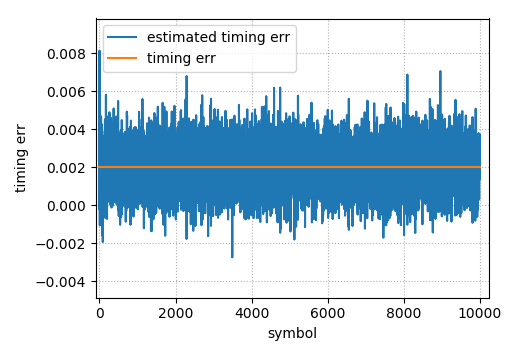
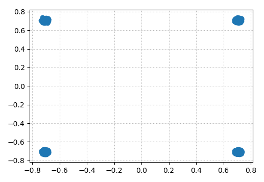
Figs. 40 and 41 show the results from the demo. The estimated error converges to 0.002 (100e-6*20) quickly. And the estimated symbols are converged to QPSK constellation well.