basics of digital signal processing

1 Basics

In this section, we will review some basic principles in digital signal processing, which will be widely used in the following sections.

1.1 Why Digital System

Fig. 1 shows a naive continuous (analog) system. It is comprised of three components: input signal $x(t)$, processing $h_t$, and output signal $y(t)$. Here, the analog signal means:

signal is continuous in time domain;
its amplitude is continuous too.

./image/comm_cont0.svg — Fig.1. Illustration of a naive communication system.

Conceptually, all processing can be done in analog domain. However, such procedure has many challenges. For example, in Fig. 2, the input $x(t)$ is multiplied by $\cos(2\pi ft)+j\sin(2\pi ft)$:

$$ \begin{align} y(t) &= y_i(t) + jy_q(t),\nonumber\\ y_i(t) &= x(t)\cos(2\pi ft),\nonumber\\ y_q(t) &= x(t)\sin(2\pi ft). \end{align} $$

./image/comm_cont1.svg — Fig.2. Modulate the signal $x(t)$ to carrier $f$ in analog domain.

The input $x(t)$ is split into two paths: one is multiplied by $\cos(2\pi ft)$, and the other is multiplied by $\sin(2\pi ft)$. Ideally, these two reference signals needs to have:

same frequency (e.g., $f$),
same amplitude (e.g, $1$),
$90^{\circ}$ phase difference.

In practice, these reference signals will never be ideal. For example, they may have amplitude mismatch, as shown in Fig. 3

$$ \begin{align} y(t) &= y_i(t)+ jy_q(t)\nonumber\\ &= x(t) (\cos(2\pi ft) + j(1+\Delta A) \sin(2\pi ft))\nonumber\\ &= x(t)(\cos(2\pi ft)+ j\sin(2\pi ft) + j\Delta A \sin(2\pi ft))\nonumber\\ &= x(t)e^{j\pi ft} + \frac{\Delta A}{2}x(t)(e^{j\pi ft} - e^{-j\pi ft}), \end{align} $$

where the first term is the desired signal, and the second term is the distortion.

./image/comm_cont2.svg — Fig.3. Modulate the signal $x(t)$ to carrier $f$ in analog domain with amplitude mismatch.

Similarly, any mismatch in phase or frequency will also cause distortion to the output signal.

If it does not sound challenging, consider a system with $N$ inputs ($x_i(t)$, $i=[1,2,\cdots, N]$), and each one is multiplied by $e^{j2\pi f_i(t)}$, respectively. Now, the system requires to keep the amplitudes, frequencies and phases of all reference signals ($\cos(2\pi f_it)$, $\sin(2\pi f_it)$) for all the time. That's one major reason OFDM (Orthogonal Frequency Division Multiplexing)¹ was not widely applied until such a process can be achieved with FFT in digital domain.

./image/comm_analog.svg — Fig.4. Modulate the $N$ signals to $N$ carrier in analog domain.

How can digital signal help in this case? In digital domain, all analog signals are first sampled every $T_s = \frac{1}{f_s}$ seconds, where $f_s$ is the sampling frequency; that is

$$ \begin{align} x_i[n] &= x_i(nT_s),\nonumber\\ \cos_i[n] &= \cos(2\pi f_i nT_s),\nonumber\\ \sin_i[n] &= \sin(2\pi f_i nT_s). \end{align} $$

Then, a 'computer' can be used to store these digital values, and do all the processing. There is no frequency, phase or amplitude mismatch in these reference signals since now they are all deterministic and stored in a computer, instead of being generated by some analog device (Fig. 5).

./image/comm_discrete.svg — Fig.5. Illustration of a naive communication system.

Of course, this is not the only advantage of the digital signal processing. For example, digital signal makes the error correction possible.

1.2 Sampling Theorem

Fig. 6 shows a digital signal processing system. Compared to Fig. 1, it has two more blocks. First, the input signal $x(t)$ is sampled (e.g., every $T_s$ second) and quantized to get a digital signal $x[n]$, so that the signal processing $h$ can be achieved in digital domain. Finally, the digital output $y[n]$ is converted to analog signal.

./image/comm_dsct.svg — Fig.6. Illustration of a digital signal processing system: (1) the analog signal is sampled, (2) the digital signal is processed; (3) the output digital signal is converted to analog domain.

Fig. 7 shows the analog sinusoid signal and its discrete time signal by sampling every $T_s$ seconds. The red dots shows the discrete values after sampling. The two analog signals (shown as blue and green curves, respectively) result in the same discrete time signal. In other words, in discrete domain, they are identical, although in analog domain, they are totally different. This causes the ambiguity, that is, the discrete time signal does not uniquely determine one analog signal.

./image/sampling_ambiguity.svg — Fig.7. The analog sinusoid signal (solid) is sampled every $T_s$ seconds to get its discrete version.

How could we make a one-to-one mapping between the discrete and analog signals? To answer this question, let us see what the discrete signal will look like after sampling. First, define a sampling sequence

$$ \begin{align} s(t) = \sum_{n=-\infty}^{\infty}{\delta(t-nT_s)}, \end{align} $$

where $\delta(t)$ is the Dirac delta function. Then,

$$ \begin{align} x_s(t) &= x(t)s(t)\nonumber\\ &= x(t) \sum_{n=-\infty}^{\infty}{\delta(t-nT_s)}\nonumber\\ &= \sum_{n=-\infty}^{\infty}{x(nT_s)\delta(t-nT_s)}. \label{eqn:sampling} \end{align} $$

Do you see how to get $x[n]$ from $x_s(t)$, and visa versa?

Eq. (\ref{eqn:sampling}) shows that $x_s(t)$ is the production of two signals $x(t)$ and $s(t)$. In frequency domain, $X_s(f)$ is the convolution between $X(f)$ and $S(f)$, that is [1]

$$ \begin{align} s(t) &\rightleftharpoons S(f),\nonumber\\ x(t) &\rightleftharpoons X(f),\nonumber\\ x_s(t) &\rightleftharpoons X_s(f),\nonumber\\ \end{align} $$

then,

$$ \begin{align} X_s(f) &= \frac{1}{2\pi}S(f)\ast X(f)\nonumber\\ &= \frac{1}{2\pi}\frac{2\pi}{T_s}\sum_{k=-\infty}^{\infty}{\delta(f-kf_s)}\ast X(f)\nonumber\\ &= \frac{1}{T_s}\sum_{k=-\infty}^{\infty}{X(f-kf_s)}. \label{eqn:sampling_freq} \end{align} $$

In other words, the frequency response of the discrete signal is the combination of the original analog signal and its shifted copies (i.e., shifted by $kf_s$). Fig. 8 shows the frequency response of the discrete signal. From this frequency response, can we determine the frequency response of the original analog signal?

./image/sampling_dsct.svg — Fig.8. Frequency response of the discrete signal.

Unfortunately, we can't. For example, as shown in Fig. 9, if the frequency response of the analog signal is either green line or blue line, its discrete signal will be same as shown in Fig. 8, when sampled at $f_s$. Take some time to convince yourself, and can you find some other frequency response that will generate the same discrete signal?

./image/sampling_analog.svg — Fig.9. Frequency response of the discrete signal.

For the example shown in Fig. 7, if the frequency of the green signal is $f_g = 1Hz$, then the frequency of the blue signal is $f_b = 6Hz$, and the sampling frequency is $f_s = 5Hz$. Then, $f_b-f_s = 6 - 5 = 1Hz = f_g$. Thus, they generates the same discrete signal.

So how to avoid such ambiguity? When we have a discrete signal, if we limit its original analog signal frequency to $[-fs/2, fs/2]$, then the analog signal is unique.

./image/sampling_dsct2.svg — Fig.10. Frequency response of the discrete signal. Solid line shows the frequency response of its corresponding analog signal, and the dotted lines are the mirrors from sampling.

There is still a problem. How can we guarantee that the frequency response of the discrete signal within $[-f_s/2, fs/2]$ is same as the original analog signal? For example, as shown in Fig. 11, the mirror frequency response at $f_s$ will overlap with the base signal (green line). In this case, the frequency response of the discrete signal within $[-fs/2,fs/2]$ will be different from the original analog signal (green line). Such phenomenon is called aliasing.

./image/sampling_alias.svg — Fig.11. Frequency response of a discrete signal withing aliasing.

Why is aliasing not good? Without aliasing, the discrete still keeps an exact copy of the original analog signal in frequency domain. Intuitively, we may be able to recover the analog signal from the discrete signal (e.g., $x[n]\rightarrow x_s(t)\rightarrow x(t)$). However, with aliasing, the original signal is distorted, and can not be recovered.

So the next question is how to avoid aliasing? Fig. 10 shows that if the signal bandwidth is $B$, then the lowest frequency component of mirror signal at $f_s$ is $f_s-B$. Thus, if $f_s-B>B$, the frequency response within $[-f_s/2, fs/2]$ will not be overlapped with other mirrors, thus, no aliasing. In particular

$$ \begin{align} f_s>2B. \label{eqn:nyquist_sampling} \end{align} $$

It is called the Nyquist sampling theorem. Eq. (\ref{eqn:nyquist_sampling}) tells us the absolute minimum of the sampling frequency. In practice,the sampling frequency is usually much higher. One reason is that if sampling frequency is close to $2B$, the transition band of the anti-aliasing filter will be extremely small, which makes the filter impractical.

To test whether you understand the sampling theorem, what's the minimal sampling frequency of the following signal? Is it $2Hz$? (Hint: what's the frequency component of a triangle signal with period $1Hz$?)

./image/sampling_triangle.svg — Fig.12. Triangle signal with period 1s.

1.3 LTI System

A system $f$ is called a linear system if and only if (iff)

$$ \begin{align} a_1f(x_1(n)) + a_2f(x_2(n)) = f(a_1x_1(n) + a_2x_2(n)). \label{eqn:linear} \end{align} $$

Similarly, a system $f$ is a time invariant system iff

$$ \begin{align} y(n) = f(x(n)) \Rightarrow y(n-n_0) = f(x(n-n_0)), \label{eqn:time_invar} \end{align} $$

for every input $x(n)$ and every time shift $n_0$.

Dirac delta function. For LTI system, one of the most important signal is Dirac delta function ($\delta[n]$) (Fig. 13)

$$ \begin{align} \delta[n] = \begin{cases} 1, & \mbox{if } n=0\\ 0, & \mbox{otherwise} \end{cases}. \end{align} $$

./image/delta.svg — Fig.13. Illustration of impulse function $\delta[n]$ ($-4 \leq n \leq 4$).

Then, any discrete signal $x[n]$ can be represented by $\delta[n]$

$$ \begin{align} x[n] = \sum_{k=-\infty}^{\infty}{x[k]\delta[n-k]}. \end{align} $$

The output of the LTI system $f$ is

$$ \begin{align} f(x[n]) &= f\left(\sum_{k=-\infty}^{\infty}{x[k]\delta[n-k]}\right) \nonumber\\ &= \sum_{k=-\infty}^{\infty}{f(x[k]\delta[n-k])}\nonumber\\ &= \sum_{k=-\infty}^{\infty}{x[k]f(\delta[n-k])}, \label{eqn:convol} \end{align} $$

where the second and third equations come from the fact that the system $f$ is a linear system. From Eq. (\ref{eqn:time_invar}), $f(\delta[n-k])$ is just a shifted copy of $f(\delta[n])$. Thus, once we know $f(\delta[n])$, we can easily write down the output of any input signal. $f(\delta[n])$ is called the impulse response of the LTI system $f$, which is usually denoted by $h[n]$. Thus, Eq. (\ref{eqn:convol}) can be written as

$$ \begin{align} f(x[n]) &= \sum_{k=-\infty}^{\infty}{x[k]f(\delta[n-k])}\nonumber\\ &= \sum_{k=-\infty}^{\infty}{x[k]h[n-k]}\nonumber\\ &:= x[n]\ast h[n], \label{eqn:convol2} \end{align} $$

where $A\ast B$ is the convolution between $A$ and $B$. So once $h[n]$ is known, the output of the LTI system can be easily got by taking the convolution between the input $x[n]$ and the impulse response $h[n]$. In other words, $h[n]$ contains all the information about the system.

If the input signal $x[n]$ is sent to multiple LTI systems in serial, for example, $f_1$ and $f_2$, then it can be shown that $x[n]\rightarrow f_1 \rightarrow f_2$² is equal to $ x[n]\rightarrow f_2 \rightarrow f_1$. Can you prove it with convolution?

Eigen Function. For an LTI system, if its input is a sinusoid (e.g., $e^{j\omega nT}$), then its output will also be a sinusoid with the same frequency (the amplitude and/or phase may change). For LTI system, we have

$$ \begin{align} f(e^{j\omega(n-n_0)T}) &= f(e^{j\omega nT}e^{-j\omega n_0T})\nonumber\\ &= f(e^{j\omega nT})e^{-j\omega n_0T}, \end{align} $$

for any time shift $n$ and $n_0$. Letting $n=0$, we have

$$ \begin{align} f(e^{j\omega(-n_0)T}) = f(1)e^{-j\omega n_0T}. \end{align} $$

Finally, letting $n_0=-n$,

$$ \begin{align} f(e^{j\omega nT}) = f(1)e^{j\omega nT}. \end{align} $$

Thus, the output of an LTI system with sinusoid input is a sinusoid with the same frequency, although the amplitude and phase may be changed. That's also the main reason that sinusoid is used in Fourier transform.

Discrete Time Fourier Transform. The discrete time Fourier transform of a discrete sequence $x[n]$ is defined as:

$$ \begin{align} X(\omega) = \sum_{n=-\infty}^{\infty}x[n]e^{-j\omega n}. \label{eqn:fourier_trans} \end{align} $$

Take the discrete time Fourier transform on Eq. (\ref{eqn:convol2}),

$$ \begin{align} \sum_{n=-\infty}^{\infty}{f(x[n])e^{-j\omega n}} &= \sum_{n=-\infty}^{\infty}{\sum_{k=-\infty}^{\infty}{x[k]h[n-k]e^{-j\omega n}}}\nonumber\\ &= \sum_{k=-\infty}^{\infty}{\sum_{n=-\infty}^{\infty}{x[k]h[n-k]e^{-j\omega n}}}\nonumber\\ &= \sum_{k=-\infty}^{\infty}{x[k]e^{-j\omega k}\sum_{n=-\infty}^{\infty}{h[n-k]e^{-j\omega (n-k)}}}\nonumber\\ &= X(\omega)H(\omega). \end{align} $$

In other words, in frequency domain, the output of the LTI system $f$ is simply the multiplication between the input and the impulse response. It is critical to digital signal processing. For example, to design a filter, we can simply focus on the $H(\omega)$.

1.4 FIR Filter

Many digital signal processing tasks can be solved by designing a filter. For example, a low pass filter can be used to filter the high frequency noise before down sampling the signal. Filters are generally grouped into two categories: finite impulse response (FIR) and infinite impulse response (IIR) filters. In this section, we will discuss the FIR. As indicated by its name, the impulse response of an FIR filter is finite. In other words, the output of an FIR filter with an impulse as its input will be zero after a finite number of samples. Fig. 14 shows the traditional tapped-delay line FIR structure (order $N$), which can be written as

$$ \begin{align} y[n] &= \sum_{k=n}^{n-N}{x[k]h[n-k]}, \end{align} $$

$$ \begin{align} y[n] &= \sum_{k=0}^{N}{x[n-k]h[k]}, \end{align} $$

where the order is defined as the maximum delay (in samples). If $x[n] = \delta[n]$, it is easy to see $y[0] = h[0]$, $y[1] = h[1]$, $\cdots$, $y[N] = h[N]$, $y[N+1] = 0$, $\cdots$, which is expected since $h$ is the impulse response of the filter by definition.

./image/filter_fir.svg — Fig.14. FIR filter structure.

Fig. 15 shows the transposed FIR filter structure. It can be obtained from the traditional tapped-delay line FIR structure by,

convert the signal nodes (the thick dot) to adders;
convert adders to signal nodes;
reverse the direction of all connections;
swap input ($x[n]$) and output ($y[n]$);
re-arrange the structure such that the input is on the left side.

./image/filter_fir_transpose.svg — Fig.15. Transposed FIR filter structure.

As we can see from Figs. 14 & 15, these two structures requires the same number of multiplications, additions and buffers (delay unit). For the transposed structure, the buffered data is after the multiplication, which usually has more bit-width in fixed-point design, and requires larger buffer size. On the other hand, in the transposed structure, the result after each adder is buffered, which may be preferred in high speed hardware implementation (e.g., FPGA), as it reduces the time required to perform multiple addition operations (in traditional structure) [2].

Bonded Input Bounded Output. An LTI system (e.g., FIR filter) is stable if for any bonded-input, its output is also bounded. In other words, for any bonded input (e.g., $|x[n]|<M_x$, $\forall n$), $|y[n]|<\infty$ if and only if $\sum_{k=0}^{N}{|h[k]|}<\infty$.

Sufficient. If $\sum_{k=0}^{N}{|h[k]|}<\infty$, then
$$ \begin{align} |y[n]| &= \left|\sum_{k=0}^{N}{x[n-k]h[k]}\right|\nonumber\\ &\leq M_x\sum_{k=0}^{N}{|h[k]|}\nonumber\\ &< \infty. \end{align} $$
Thus, the output $y[n]$ is bounded.
Necessary. If the output $y[n]$ is bounded, in other words $|y[n]|<\infty$ $\forall n$ for any bounded input $x[n]$. Let $x[n-k] = \textrm{sign}(h[k])$, where
$$ \begin{align} \textrm{sign}(A) = \begin{cases} 1, & \mbox{if } A\geq0 \\ -1, &\textrm{otherwise}. \end{cases} \end{align} $$
It is easy to see $x[n]$ is bounded. So, $y[n]$ is also bounded, that is
$$ \begin{align} |y[n]| &= \left|\sum_{k=0}^{N}{x[n-k]h[k]}\right|\nonumber\\ & = \left|\sum_{k=0}^{N}{|h[k]|}\right|\nonumber\\ & = \sum_{k=0}^{N}{|h[k]|}\nonumber\\ &<\infty. \end{align} $$

Thus, FIR filter is always stable since its number of coefficients is limited (as long as its coefficients are finite). It may not be true for IIR filters as shown below. However, such feature is not free since generally FIR needs more multiplications than IIR to achieve similar performance.

Causality. The general equation for FIR is

$$ \begin{align} y[n] &= \sum_{k=-M}^{N}{x[n-k]h[k]}\nonumber\\ &= \cdots + x[n-1]\times h[1] + x[n]\times h[0] + x[n+1]\times h[-1] + \cdots. \end{align} $$

where $M\geq 0$, $N\geq 0$. In practice, such filter is infeasible, since it needs to know future inputs $x[n+1]$, $x[n+2]$, $\cdots$ to calculate the current output $y[n]$. That is, the filter is non-casual (the current output is determined by the future inputs). One solution is to introduce some delay to make the filter casual. For example, considering the non-casual filter

$$ \begin{align} y[n] &= \sum_{k=-M}^{N}{x[n-k]h[k]} &\Rightarrow \nonumber\\ y[n-M] &= \sum_{k=-M}^{N}{x[n-M-k]h[k]}&\Rightarrow\nonumber\\ y[n-M] &= \sum_{k=0}^{N+M}{x[n-k]h[k-M]}. \label{eqn:fir} \end{align} $$

Let $y'[n] = y[n-M]$, $h'[k] = h[k-M]$, Eq. (\ref{eqn:fir}) can be written as

$$ \begin{align} y'[n] = \sum_{k=0}^{N+M}{x[n-k]h'[k]}. \end{align} $$

In this case, the filter defined by $h'[k]$ is a casual filter ($y^\prime[n]$ only depends on the current and previous input samples), which introduces $M$ samples delay in both the filter coefficients and the outputs. For simplicity, we will also use $y[n]$ and $h[n]$ to indicate the output and coefficients of the causal FIR filter

$$ \begin{align} y[n] = \sum_{k=0}^{N+M}{x[n-k]h[k]}. \end{align} $$

Group Delay. Let's assume the coefficients in Eq. (\ref{eqn:fir}) is symmetric; that is $h[-k]=h[k]$, and $M=N$. In this case, its frequency response is real

$$ \begin{align} H(\omega) &= \sum_{k=-N}^{N}{h[k]e^{-j\omega k}}\nonumber\\ &= h[0] + \sum_{k=1}^{N}{h[k]e^{-j\omega k}+h[-k]e^{-j\omega(-k)}}\nonumber\\ &= h[0] + \sum_{k=1}^{N}{h[k](e^{-j\omega k}+e^{-j\omega(-k)})}\nonumber\\ &= h[0] + \sum_{k=1}^{N}{2h[k]\cos(\omega k)}. \end{align} $$

For a causal filter $h'[k] = h[k-N]$

$$ \begin{align} H'(\omega) &= \sum_{k=0}^{2N}{h'[k]e^{-j\omega k}}\nonumber\\ &= \sum_{k=0}^{2N}{h[k-N]e^{-j\omega k}}\nonumber\\ &\stackrel{k'=k-N}{=} \sum_{k'=-N}^{N}{h[k']e^{-j\omega (k'+N)}}\nonumber\\ &= \sum_{k'=-N}^{N}{h[k']e^{-j\omega (k'+N)}}\nonumber\\ &= e^{-j\omega N} H(\omega). \end{align} $$

And for input $x[n]=e^{j\omega_xn}$, the frequency response is:

$$ \begin{align} X(\omega) = 2\pi\sum_{k=-\infty}^{\infty}{\delta(\omega-\omega_x-2k\pi)} \end{align}. $$

And its output is

$$ \begin{align} Y'(\omega) &= 2\pi\sum_{k=-\infty}^{\infty}{\delta(\omega-\omega_x-2k\pi)} H'(\omega)\nonumber\\ &= 2\pi\sum_{k=-\infty}^{\infty}{\delta(\omega-\omega_x-2k\pi)} e^{-j\omega N} H(\omega)\nonumber\\ &= e^{-j\omega_x N} H(\omega_x) 2\pi\sum_{k=-\infty}^{\infty}{\delta(\omega-\omega_x-2k\pi)}. \end{align} $$

In time domain

$$ \begin{align} y'[n] &= e^{-j\omega_x N} H(\omega_x)e^{j\omega_xn}\nonumber\\ & =H(\omega_x)e^{j\omega_x(n-N)}. \end{align} $$

Thus,

$$ \begin{align} x[n]=e^{j\omega_xn} \stackrel{h}{\longrightarrow} y'[n] = H(\omega_x)e^{j\omega_x(n-N)}. \end{align} $$

In other words, compared to the input, the output is delayed by $N$ samples, and the magnitude is scaled by $ H(\omega_x)$. Since $\omega_x$ is arbitrary, the delay is same for all frequency components, which is donated as group delay:

$$ \begin{align} \tau(\omega) &= \frac{-\partial \phi(H'(\omega))}{\partial \omega}\nonumber\\ &= \frac{-\partial (-\omega N)}{\partial \omega}\nonumber\\ &= N. \end{align} $$

It is a general definition of group delay of a system. And in most practice case, the FIR filter you designed will be symmetric and the group delay can easily calculated as $(N_{\textrm{FIR}}-1)/2$, where $N_{\textrm{FIR}}$ is the number of filter coefficients.

Prove $(N_{\textrm{FIR}}-1)/2$ is also true when $N_{\textrm{FIR}}$ is an even number.

For a general FIR filter, it is a little bit complicate. For example, how to calculate the group delay of the filter with coefficients $[M, M-1,\cdots, 1]$? Without lose of generality, let a filter have coefficients $[b_0, b_1, \cdots, b_{M-1}]$. Then the filter output is

$$ \begin{align} y[n] = b_0 x[n] + b_1x[n-1] + \cdots + b_{M-1}x[n-M+1]. \end{align} $$

Thus, the frequency response of the transfer function can be written as

$$ \begin{align} H(\omega) &= b_0 + b_1e^{-j\omega} + \cdots + b_{M-1}e^{-j\omega(M-1)}\nonumber\\ &= H_r(\omega) + jH_i(\omega), \end{align} $$

where

$$ \begin{align} H_r(\omega) &= b_0 + b_1\cos(\omega) + \cdots + b_{M-1}\cos(\omega(M-1)),\nonumber\\ H_i(\omega) &= -(b_1\sin(\omega) + \cdots + b_{M-1}\sin(w(M-1))). \end{align} $$

Thus the phase can be written as

$$ \begin{align} \phi(\omega) = \textrm{atan}\left(\frac{H_i(\omega)}{H_r(\omega)}\right). \end{align} $$

And the delay is

$$ \begin{align} \tau(\omega) &= -\frac{ \partial \phi(\omega)}{\partial \omega}\nonumber\\ &= -\frac{1}{1+(\frac{H_i(\omega))}{(H_r(\omega))})^2}\left(\frac{H_i(\omega)^\prime}{H_r(\omega)} - \frac{H_i(\omega)H_r(\omega)^\prime}{H_r(\omega)^2}\right), \end{align} $$

where $H_i(\omega)^\prime$ and $H_r(\omega)^\prime$ are $\frac{\partial H_i(\omega)}{\partial \omega}$, $\frac{\partial H_r(\omega)}{\partial \omega}$, respectively. The delay at $\omega=0$ is

$$ \begin{align} \tau(0) &= -\frac{1}{1+(\frac{H_i(0)}{H_r(0)})^2}\left(\frac{H_i(0)^\prime}{H_r(0)} - \frac{H_i(0)H_r(0)^\prime}{H_r(0)^2}\right)\nonumber\\ &= -\frac{H_i(0)^\prime}{H_r(0)}\nonumber\\ &= \frac{b_1+2b_2 +\cdots+ (M-1)b_{M-1}}{b_0+b_1+b_2+\cdots+b_{M-1}}. \label{eqn:delay_fir} \end{align} $$

Thus for filter with coefficients $[M, M-1, \cdots, 1]$,

$$ \begin{align} \tau(0) &= \frac{(M-1)+(M-2)*2+\cdots+1*(M-1)}{M(M+1)/2}\nonumber\\ &= \frac{M-1}{3}. \label{eqn:groupdelay_example1} \end{align} $$

>>> from scipy import signal, pi
>>> b = list(range(10, 0, -1))
>>> w, gd = signal.group_delay((b, 1))
>>> import matplotlib.pyplot as plt
>>> plt.plot(w/pi/2, gd)
>>> plt.ylabel('Group delay (samples)')
>>> plt.xlabel('Normalized frequency')
>>> plt.grid('on', ls='dotted')
>>> plt.xlim([0, 0.5])
>>> plt.show()

./image/groupdelay.svg — Fig.16. Group delay of FIR filter with coefficients $[10,9, \cdots, 1]$. The $x$-axis is the frequency normalized to sampling frequency ($f_n = f/f_s$).

As shown in Fig. 16, the group delay at normalized frequency $f_n=0$ is $3$ samples, which matches with Eq. (\ref{eqn:groupdelay_example1}). In other words, for the input signal near $f_n = 0$, the output will be delayed by 3 samples.

What happens at normalized frequency $f_n \approx 0.1$, where the group delay is negative (e.g., $\approx$ -2)? Following the above group delay definition, it means that there is a time advance between the output and input. So, does it mean we actually create a non-causal system with a casual filter? The answer is no. As we know, for narrow band (band limited) signal, its current signal may be predicted by the previous samples. So at $f_n \approx 0.1$, the filter tries to predict the inputs from its previous samples, which causes an illusion of time advance (further reading).

Implementation considerations. The general equation of an FIR filter is,

$$ y[n] = x[n]h[0] + x[n-1]h[1] + x[n-2]h[2] + \cdots + x[n-N+1]h[N-1], \label{eqn:fir_imp} $$

where $N$ is the filter length. So for each input sample, it needs $N$ multiplications and $N-1$ additions to calculate the output. However, in practice, the coefficients of most FIR filter will be symmetric around the center coefficient, that is $h[n]=h[N-1-n], \forall n$. Thus, Eq. (\ref{eqn:fir_imp}) can be written as

$$ y[n] = (x[n]+x[n-N+1])h[0] + (x[n-1]+x[n-N+2]))h[1] + \cdots, \label{eqn:fir_imp_symmetric} $$

In this case, it only needs $\sim \frac{N}{2}$ multiplications and $N-1$ additions to calculate output $y[n]$.

One special case is half band filter, which can be implemented more efficiently. To see how it works, assume its $2N+1$ coefficients are real ($[h[0],h[1],\cdots,h[2N]$), and symmetric $h[n] = h[2N-n]$. Thus, the frequency response is

$$ \begin{align} H(f) &= \sum_{n=0}^{2N}{h[0]e^{-j2\pi nf}}\nonumber\\ &= \sum_{n=0}^{N-1}{h[n](e^{-j2\pi nf}+e^{-j2\pi (2N-n)f})} + h[N]e^{-j2\pi Nf}\nonumber\\ &= \sum_{n=0}^{N-1}{e^{-j2\pi Nf}h[n](e^{-j2\pi (n-N)f}+e^{-j2\pi (N-n)f})} + h[N]e^{-j2\pi Nf}\nonumber\\ &= e^{-j2\pi Nf}\left(\sum_{n=0}^{N-1}{2h[n]\cos(2\pi(N-n)f)} + h[N]\right). \end{align} $$

And its magnitude is

$$ \begin{align} \left|H(f)\right| = \sum_{n=0}^{N-1}{2h[n]\cos(2\pi(N-n)f)} + h[N]. \end{align} $$

Let $|H(0.25-f)|+|H(0.25+f)| = 1$. Thus

$$ \begin{align} &\frac{\partial |H(0.25-f)|+|H(0.25+f)|}{\partial f} \nonumber\\ &= \sum_{n=0}^{N-1}{4\pi h[n](N-n)(\sin(2\pi(N-n)(0.25-f))-\sin(2\pi(N-n)(0.25+f)))}\nonumber\\ & \equiv 0 \label{eqn:fir_halfband} \end{align} $$

So, if $N-n$ is odd,

$$ \begin{align} \sin(2\pi(N-n)(0.25-f))-\sin(2\pi(N-n)(0.25+f)) = 0, \end{align} $$

if $N-n$ is even,

$$ \begin{align} \sin(2\pi(N-n)(0.25-f))-\sin(2\pi(N-n)(0.25+f)) = 2\sin(2\pi(N-n)(0.25-f)). \end{align} $$

Thus, to make Eq. (\ref{eqn:fir_halfband}) hold for all $f$, $h[n]=0$ when $N-n$ is even. In other words, roughly half of the coefficients are zero! For example

>>> scipy.signal.firwin(11, 0.5)
array([  5.06031712e-03,  -3.25061549e-18,  -4.19428794e-02,
         1.32104345e-17,   2.88484826e-01,   4.96795472e-01,
         2.88484826e-01,   1.32104345e-17,  -4.19428794e-02,
        -3.25061549e-18,   5.06031712e-03])

Thus, it only needs roughly $N/4$ multiplications and $N/2$ additions to calculate the output.

Another special case is polyphase filter, which will be discussed later. In such case, the computation complexity can be further decrease by

not calculating the output that will be discard by the following block,
not calculating the multiplication when the input is zero.

So far, we are focusing on reducing the number of multiplications. It makes sense for many hardware implementations (e.g., ASIC or FPGA), where multiplications is expensive (e.g., area, time). Occasionally, you may also needs to implement the filter in pure software. Here software is not something like Matlab, Scilab, or scipy, where you may always have access to some efficient pre-defined functions. For example, you may need to implement an FIR filter on a ARM MCU. As shown in Fig. 17, at each input sample, you will need to calculate the multiplications between input samples $x[n]$ and filter coefficients $h[n]$, then shift the current input to the buffer.

Fig.17. Operations for FIR filter at each input sample.

For some implementations, Shift input to buffer operation may also be expensive. For example, for a filter with length $N$, at $n^{th}$ sample, $x[n]$ is move to $b[0]$, $x[n-1]$ is moved from $b[0]$ to $b[1]$, $\cdots$, $x[n-N+1]$ is moved to $x[N-1]$, while $x[n-N]$ is discarded.

As shown in FirAlgs.c, there are several ways to handle this. The naive solution may look like³

SAMPLE fir_basic(SAMPLE input, int ntaps, const SAMPLE h[], SAMPLE z[])
{
    int ii;
    SAMPLE accum;

    /* store input at the beginning of the delay line */
    z[0] = input;

    /* calc FIR */
    accum = 0;
    for (ii = 0; ii < ntaps; ii++) {
        accum += h[ii] * z[ii];
    }

    /* shift delay line */
    for (ii = ntaps - 2; ii >= 0; ii--) {
        z[ii + 1] = z[ii];
    }

    return accum;
}

It basically has two for loops. The first one is to calculate the output (multiplications and additions). The second one is to shift the input samples, which can be eliminated by using a circular buffer.

SAMPLE fir_circular(SAMPLE input, int ntaps, const SAMPLE h[], SAMPLE z[],
                    int *p_state)
{
    int ii, state;
    SAMPLE accum;

    state = *p_state;               /* copy the filter's state to a local */

    /* store input at the beginning of the delay line */
    z[state] = input;
    if (++state >= ntaps) {         /* incr state and check for wrap */
        state = 0;
    }

    /* calc FIR and shift data */
    accum = 0;
    for (ii = ntaps - 1; ii >= 0; ii--) {
        accum += h[ii] * z[state];
        if (++state >= ntaps) {     /* incr state and check for wrap */
            state = 0;
        }
    }

    *p_state = state;               /* return new state to caller */

    return accum;
}

Now it only has one for loop, and no need to shift the input samples. However, in this for loop, it needs to check the index overflow of the buffer, which is also expensive.

In this case, we can use two filter coefficients copies to avoid checking the buffer index inside the loop. For example, assume the filter coefficients are $h[0] \sim h[4]$, and the inputs are $x[0]$, $x[1]$, $x[2]$, $\cdots$. Since the number of the filter coefficients is 5, we need to have a buffer of length 5 to hold all the inputs, and a buffer of length 10 to hold two copies of the filter coefficients⁴. Fig. 18 shows the buffer status when the first input $x[0]$ arrives. $x[0]$ is stored at position 0 of the data buffer, i.e., $b[0]$.

./image/filter_fir_dbl_h0.svg — Fig.18. Status of buffers with double filter coefficients filtering, when $x[0]$ arrives.

To calculate the filter output, align $b[0]$ with $h[0]$ (as show in Fig. 18), that is

$$ \begin{align} y[0] &= h[0] x[0] + h[1]\times 0 + h[2] \times 0 + h[3]\times 0 + h[4]\times 0\nonumber \\ &= h[0]x[0]. \end{align} $$

When the next input $x[1]$ arrives, it will be stored at position $0-1 = 4 (\textrm{mod 5})$ of the input buffer, rather than shifting $x[0]$. The buffer will look like

./image/filter_fir_dbl_h1.svg — Fig.19. Status of buffers with double filter coefficients filtering, when $x[1]$ arrives.

In naive implementation, we want the correlation to be done as

./image/filter_fir_dbl_h2.svg — Fig.20. Naive filtering buffer status, when $x[1]$ arrives.

Fortunately, in double filter coefficients implementation, it can be achieved by aligning the data buffer and the filter coefficients buffer,

./image/filter_fir_dbl_h3.svg — Fig.21. Align the filter coefficients buffer with data buffer properly for multiplication, when $x[1]$ arrives.

In other words, align the 1st element of data buffer with the 2nd element of the filter coefficients buffer. Then the multiplication and summation is done on two continuous buffers. In some MCU, it can be implemented efficiently. And due to the double copies of the filter coefficients, there is no need to check the overflow of the filter coefficients buffer. It is easy to see that

$$ \begin{align} y[1] &= h[1] \times x[0] + h[2] \times 0 + h[3] \times 0 + h[4] \times 0 + h[0] \times x[1]\nonumber \\ &= h[1]x[0]+h[0]x[1], \end{align} $$

which is same as the multiplication result from Fig. 20.

Similarly, for 3rd inputs $x[2]$, it will be stored at position $4-1=3$ of data buffer, and the correlation can be done by aligning the input and filter coefficients buffer as

./image/filter_fir_dbl_h4.svg — Fig.22. Align the filter coefficients buffer and data buffer properly for multiplication, when $x[2]$ arrives.

One possible implementation may look like

SAMPLE fir_double_h(SAMPLE input, int ntaps, const SAMPLE h[], SAMPLE z[],
                    int *p_state)
{
    SAMPLE accum;
    int ii, state = *p_state;
    SAMPLE const *p_h, *p_z;

    /* store input at the beginning of the delay line */
    z[state] = input;

    /* calculate the filter */
    p_h = h + ntaps - state;
    p_z = z;
    accum = 0;
    for (ii = 0; ii < ntaps; ii++) {
        accum += *p_h++ * *p_z++;
    }

    /* decrement state, wrapping if below zero */
    if (--state < 0) {
        state += ntaps;
    }
    *p_state = state;       /* return new state to caller */

    return accum;
}

Fixed-point design. So far all we discussed is based on the implementation with float/double values. In other words, the bit-width is much more than required. In some implementations, it may be free to use float/double values (e.g., the float value multiplication may be done in a single cycle.). In many other implementations, float/double values is not acceptable (e.g., speed, area). In this case, you need to design the fixed-point version of the filter. We will use an example to show the general procedure. For this trivial example, define the signal and noise

>>> # normalized signal frequency
>>> fs = 0.02
>>> s = np.sin(2*np.pi*fs*np.arange(1000))
>>> # normalized noise frequency
>>> fn = 0.2
>>> n = np.sin(2*np.pi*fn*np.arange(1000))
>>> plt.clf()
>>> plt.subplot(2, 1, 1)
>>> plt.plot(s)
>>> plt.plot(n)
>>> plt.legend(['signal', 'noise'])
>>> plt.xlim([0, 100])
>>> plt.subplot(2, 1, 2)
>>> plt.plot(np.linspace(0, 1, len(s), endpoint=False), 20*np.log10(abs(np.fft.fft(s+n))))
>>> plt.xlabel('Normalized frequency')
>>> plt.show()

Next step is to make the fixed-point input. It basically relies on the system and the previous block. For example, if the previous block is an ADC, then it may have some fixed data bit-width (e.g., 8 or 10 bits per sample). For this example, we assume that each sample of input has 8 bits, and 3 bits before the decimal point. In particular, the range of the input values is $[-4, 3.96875]$⁵ with step 0.3125. Thus, as shown in the following figure, the difference between the fixed-point and float-point samples is $[-0.0156, 0.0156]$.

>>> # normalize the input signal to 8 bits (3 bits before the decimal point)
>>> r = np.round((s+n)*2**5)/2**5
>>> plt.plot(r-n-s, 'r')
>>> plt.title('difference between the float and fixed input')
>>> plt.show()

Then, we design the float point filter and apply it to the input signals.

>>> # estimate the number of filter coefficients
>>> N = np.ceil(60/22/((fn-fs))).astype(int)
>>> # design the low-pass filter
>>> b = scipy.signal.firwin(N, (fn+fs)/2)
>>> b
array([0.00235884, 0.00608626, 0.01690498, 0.03741456, 0.06652325,
       0.09912455, 0.1275165 , 0.14407105, 0.14407105, 0.1275165 ,
       0.09912455, 0.06652325, 0.03741456, 0.01690498, 0.00608626,
       0.00235884])
>>> # apply the filter to input
>>> y = scipy.signal.lfilter(b, 1, r)
>>> plt.plot(r, 'b')
>>> plt.plot(s, 'g')
>>> plt.plot(y, 'r')
>>> plt.xlim([0, 100])
>>> plt.legend(['signal+noise', 'signal', 'filtered'])
>>> plt.show()

As shown in the above figure, after the filter, the majority of the noise has been filtered out. And note there is a delay between the signal and the filtered output due to the filter.

Everything looks fine. Now we start to design the fixed-point filter. The maximum filter coefficient is 0.14407105, thus the first 2 bits after the decimal point is always zero, for example, in binary format b'.0010010011100001. So if we want the coefficients to have 8 effective bits, we will keep the coefficients from bit -3 to bit -10, i.e., b'.0010010011100001⁶. And since the 11th bit is 1, add 1 to 10th bits as we use round for truncation. Thus, the final fixed-point coefficient for 0.14407105 is b'.0010010100.

>>> Nc = 8
>>> bf = np.round(b*2**(Nc+2))/2**(Nc+2)
>>> yf = scipy.signal.lfilter(bf, 1, r)
>>> plt.plot(y-yf)
>>> plt.show()

./image/fir_demo_signal_filtered_fix.svg

So how many bits does the filter coefficients need? We can plot the difference between the results from the float-point and fixed-point filter coefficients. The actual number relies on application, for example, the error from the fixed-point filter coefficients does not dominate the total noise in the signal.

>>> mse = []
>>> NC = np.arange(4, 20)
>>> for Nc in NC:
...     bf = np.round(b*2**(Nc+2))/2**(Nc+2)
...     yf = scipy.signal.lfilter(bf, 1, r)
...     mse.append(np.sqrt(np.mean((yf-y)**2)))
>>> plt.semilogy(NC, mse, '-o')
>>> plt.grid('on', ls='dotted')
>>> plt.ylabel('MSE')
>>> plt.xlabel('# of effective bits of filter coefficients')
>>> plt.show()

./image/fir_demo_signal_filtered_fix_mse.svg

The above figure shows that roughly the MSE between the fixed and float filter results decreases when the number of the effective bits increases. It makes sense since the more the effective bits, the smaller the difference between the fixed-point and float-point values. However, the truncation will slightly changes the frequency response, which also cause the jitter along the trace. Besides the round, you may also try some other truncation method (see SystemC User Guide Chapter 7 for details).

>>> mse_f = []
>>> for Nc in NC:
...     bf = np.floor(b*2**(Nc+2))/2**(Nc+2)
...     yf = scipy.signal.lfilter(bf, 1, r)
...     mse_f.append(np.sqrt(np.mean((yf-y)**2)))
>>> plt.semilogy(NC, mse, '-o')
>>> plt.semilogy(NC, mse_f, 'r-s')
>>> plt.grid('on', ls='dotted')
>>> plt.ylabel('MSE')
>>> plt.xlabel('# of effective bits of filter coefficients')
>>> plt.legend(['round', 'floor'])
>>> plt.show()

./image/fir_demo_signal_filtered_fix_mse2.svg

One thing we haven't discussed yet is the output. For example, in above example, the input is 8 bits. If the filter coefficient is also 8 bits, the output will be 20 bits (8+8+4⁷). However, it may be not necessary to output all these 20 bits to the next block, since, for example, the LSB bits may contain only noise, and/or the MSB bits may be always zero (or sign bits). For this example, the expected output is within $[-1,1]$, it may be reasonable to have 3 bits for integers (include 1 sign bit). To quantify the signal, we need additional saturation step to make sure the output value is within its range (e.g., no overflow). It is especially important when we try to ignore the MSB bits in the result.

>>> Nc = 8
>>> bf = np.round(b*2**(Nc+2))/2**(Nc+2)
>>> yf = scipy.signal.lfilter(bf, 1, r)
>>> mse_y = []
>>> for Ny in range(3, 20):
...     yf_t = np.round(yf*2**Ny)
...     # saturation
...     yf_t[yf_t >= 2**(Ny+3-1)] = 2**(Ny+3-1)-1
...     yf_t[yf_t < -2**(Ny+3-1)] = -2**(Ny+3-1)
...     yf_t = yf_t/2**Ny
...     mse_y.append(np.sqrt(np.mean((yf_t-y)**2)))
>>> plt.semilogy(np.arange(3, 20)+3, mse_y, '-o')
>>> plt.grid('on', ls='dotted')
>>> plt.ylabel('MSE')
>>> plt.xlabel('# of effective output bits')
>>> plt.show()

./image/fir_demo_signal_filtered_fix_msey.svg

1.5 IIR Filter

As shown in the previous section, FIR filter only uses the current and previous input samples to calculate filter output. In contrast, IIR (infinite impulse response) filter will also use the previous filter outputs in calculation. The general equation may look like

$$ \begin{align} y[n] = \sum_{m=1}^{M}{a[m]y[n-m]} + \sum_{l=0}^{L}{b[l]x[n-l]}. \end{align} $$

For simplicity, when $L=M=1$, the IIR filter structure is shown in Fig. 30.

./image/filter_iir_s.svg — Fig.30. IIR filter direct form I structure.

We can interchange the left and right components to get

./image/filter_iir2_s.svg — Fig.31. IIR filter structure.

To see the filters in Figs. 30 and 31 are identical,

$$ \begin{align} w[n] &= x[n] + a[1]w[n-1]\nonumber\\ y[n] &= b[0]w[n]+b[1]w[n-1], \end{align} $$

then

$$ \begin{align} y[n] &= b[0](x[n]+a[1]w[n-1])+b[1](x[n-1]+a[1]w[n-2])\nonumber\\ &= b[0]x[n] + b[1]x[n-1]+a[1](b[0]w[n-1]+b[1]w[n-2])\nonumber\\ &=b[0]x[n] + b[1]x[n-1]+a[1]y[n-1], \label{eqn:filter_iir} \end{align} $$

which is identical to the Fig. 30. It is easy to see that both delay units in Fig. 31 store the same data $w[n-1]$. So one can be eliminated

./image/filter_iir3_s.svg — Fig.32. IIR filter direct form II structure.

As mentioned above, the FIR filter is always stable (i.e., bonded input bounded output); however, it is not true for IIR filter. For example, if $a[1]= 2$ and $b[0]=b[1]=1$, that is

$$ y[n] = 2y[n-1] + x[n]+x[n-1], $$

it is easy to see that for bounded input $x[n]=\delta(n)$, $y[n]$ approaches infinity. To see when the IIR filter is stable, let's solve the difference equations defined by Eq. (\ref{eqn:filter_iir}). First let $x[n]=0$, $\forall n$, that is

$$ \begin{align} y[n] = a[1]y[n-1], \label{eqn:iir_homogeneous} \end{align} $$

which is called homogeneous difference equation. Its general solution is $y[n] = A\lambda^n$. Substitute it into Eq. (\ref{eqn:iir_homogeneous}),

$$ \begin{align} A\lambda^n = a[1]A\lambda^{n-1}, \end{align} $$

which leads to $\lambda = a[1]$ and $y[n] = Aa[1]^n$. It is easy to see that if $|a[1]|>1$, $y[n]$ will approach infinity.

Even sometime the filter is stable, its intermittent value may approach infinity. For example, consider a filter

$$ \begin{align} y[n] = y[n-1] + x[n] - x[n-2] \end{align} $$

which is stable since it is equivalent to filter $y[n] = x[n]+x[n-1]$. However, if it is implemented as (direct II form)

$$ \begin{align} w[n] &= w[n-1]+x[n]\nonumber\\ y[n] &= w[n] - w[n-2], \end{align} $$

it is easy to see $w[n]$ is not stable. So when implementing a filter, we need to make sure all internal values are also bounded; otherwise, the filter may not work correctly.

Group delay. As shown in previous section, for FIR filter with symmetric coefficients, the group delay is a constant. In other words, each frequency component will experience a same phase delay after the filter. It is a very nice feature since the signal will not be distorted. However, it is not true for IIR filter. Thus, it is good idea to check the group delay carefully, especially when the signal bandwidth is so large that the group delay within that band may not be roughly a constant.

Fixed-point design. Let use the simplest first order IIR filter as an example.

$$ \begin{align} y[n] = \alpha \cdot y[n-1] + [1-\alpha]\cdot x[n]. \label{eqn:iir_1st} \end{align} $$

For float-point design, it may be implemented as

// Float point
float simple_iir( float x, float& yp, float alpha)
{
  // x: input sample x[n]
  // yp: the previous output y[n-1]
  // alpha: IIR filter coefficient

  // calculate the filter output
  float y = alpha*yp + (1-alpha) *x;
  // or to save one multiplication: y = alpha*(yp - x) + x;

  // save the output for next input sample
  yp = y;

  return y;
}

As usual, for fixed-point design, we need to determine the input ($x[n]$), output ($y[n]$), and the filter coefficient ($\alpha$) bit-widths. As mentioned before, this can be done with simulation. For example, we may try 6 bits input and keep the output/filter coefficients unchanged (float or double), then compared the difference between the output with the previous all float filter. If the performance is within the specification (e.g., SNR), we are done. Otherwise, try 7 bits, 8 bits..., until we are satisfied.

Once we determine the input bit-width (e.g., 10bits after decimal point, total bits 12 bits); we can continue to determine the bit-width of filter coefficients and output with same method. After all bit-widths are determined, we can implement the fixed-point IIR.

For example, if we determine that input has 10 bits after decimal point (total 12 bits); coefficient has 8 bits after decimal point (total 8 bits); output 12 bits after decimal point (total 16 bits)

$$ \begin{align} x_i[n] &= x[n]\times 2^{10}\nonumber\\ \alpha_i &= \alpha\times 2^8\nonumber\\ y_i[n] &= y[n]\times 2^{12}, \label{eqn:iir_1st_fixed_def} \end{align} $$

where $x_i[n]$, $y_i[n]$, and $\alpha_i$ are the fixed-point input, output and filter coefficient, respectively (represented by integer). Substitute Eq. (\ref{eqn:iir_1st_fixed_def}) into Eq. (\ref{eqn:iir_1st})

$$ \begin{align} y_i[n]/2^{12} &= \alpha_i/2^8\times (y_i[n-1]/2^{12} - x_i[n]/2^{10}) + x_i[n]/2^{10} \Rightarrow\nonumber\\ y_i[n]\times 2^8 &= \alpha_i\times (y_i[n-1] - x_i[n]\times 2^2) + x_i[n]\times 2^{10}. \end{align} $$

int alpha_i = int(alpha*(1<<8)+0.5);
int simple_iir_i( int x_i, int& yp_i, int alpha_fixed)
{
    // x_i: input sample x_i[n]
    // yp_i: the previous output y_i[n-1]
    // alpha_i: IIR filter coefficient

    int y_i = alpha_i*(yp_i-(x_i<<2)) + (x_i<<10);

    // save the output for next input sample, here truncation is used
    yp_i = y_i>>8;
    // to check the overflow (e.g., 16 bit output, -2^15~2^15-1),  for example
    if(yp_i>=(1<<15)) yp_i = (2<<15) - 1;
    if(yp_i<-(1<<15)) yp_i = -(2<<15);

    return yp_i;
}

For the above pseudo-code, we arbitrarily use << operator, which may not be well-defined on your platform and may be replaced with multiplication.

1.6 Estimation & Detection

One important application of digital signal processing is to detect signal from noise. For example, if a received signal is

$$ \begin{align} x = s + n, \end{align} $$

where $s$ is a either 1 or -1, $n$ is noise. How to detect $s$ by receiving $x$? One reasonable idea is to check whether $x$ is more likely to be received when $s=1$ is transmitted. In other words, if the probability of receiving $x$ given $s=1$ is sent ($p(x|s=1)$) is larger than the probability of receiving $x$ given $s=-1$ is sent ($p(x|s=-1)$), then we can says that $s=1$ is transmitted, and visa versa. That is

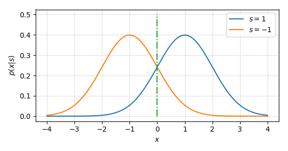
$$ \begin{align} p(x|s=1) \mathrel{\mathop\gtrless\limits^{1}_{-1}} p(x|s=-1). \label{eqn:det_binary} \end{align} $$

Eq. (\ref{eqn:det_binary}) is called ML (maximum likelihood) detection. If $n$ is AWGN (additive white Gaussian noise), both $p(x|s=1)$ and $p(x|s=-1)$ follow Gaussian distribution, i.e.,

$$ \begin{align} p(x|s=1) &= \frac{1}{\sqrt{2\pi\sigma^2}}e^{-\frac{(x-1)^2}{2\sigma^2}},\nonumber\\ p(x|s=-1) &= \frac{1}{\sqrt{2\pi\sigma^2}}e^{-\frac{(x+1)^2}{2\sigma^2}}, \end{align} $$

where $\sigma^2$ is the variance of $n$. In this case, Eq. (\ref{eqn:det_binary}) can be written as

$$ \begin{align} p(x|s=1) &\mathrel{\mathop\gtrless\limits^{1}_{-1}} p(x|s=-1) &\Rightarrow\nonumber\\ \frac{1}{\sqrt{2\pi\sigma^2}}e^{-\frac{(x-1)^2}{2\sigma^2}} &\mathrel{\mathop\gtrless\limits^{1}_{-1}} \frac{1}{\sqrt{2\pi\sigma^2}}e^{-\frac{(x+1)^2}{2\sigma^2}} &\Rightarrow\nonumber\\ e^{-\frac{(x-1)^2}{2\sigma^2}} &\mathrel{\mathop\gtrless\limits^{1}_{-1}} e^{-\frac{(x+1)^2}{2\sigma^2}} &\Rightarrow\nonumber\\ -\frac{(x-1)^2}{2\sigma^2} &\mathrel{\mathop\gtrless\limits^{1}_{-1}} -\frac{(x+1)^2}{2\sigma^2} &\Rightarrow\nonumber\\ (x-1)^2 &\mathrel{\mathop\lessgtr\limits^{1}_{-1}} (x+1)^2 &\Rightarrow\nonumber\\ x &\mathrel{\mathop\gtrless\limits^{1}_{-1}} 0. \label{eqn:det_binary_ml} \end{align} $$

Thus, the ML detection rule is very simple, that is, if $x$ is large than 0, $s=1$ is sent, otherwise $s=-1$ is sent. It can also be read from Fig. 33. For example, when $x>0$, $p(x|s=1)>p(x|s=-1)$.

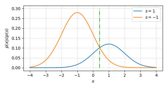
./image/basics_det_ml_prop.png — Fig.33. Conditional probability of the received signal $x$ given the transmitted signal $s$.

Such procedure may have a drawback since it does not take the probability of $s=1$ or $s=-1$ into consideration. For example, if $p(s=1)=1$ (i.e., the system keeps sending 1), the optimal detection procedure should also always determine $s=1$ is sent, instead of the one shown in Eq. (\ref{eqn:det_binary_ml}). In this case, the object function is changed to

$$ \begin{align} p(s=1|x) &\mathrel{\mathop\gtrless\limits^{1}_{-1}} p(s=-1|x). \label{eqn:det_binary_map} \end{align} $$

It is also called MAP (Maximum A Posteriori) estimation. This time, we compare the probability of $s=1$ and $s=-1$ given $x$ is received. Thanks to Bayes' theorem,

$$ \begin{align} p(s=1|x) = \frac{p(x|s=1)p(s=1)}{p(x)}. \end{align} $$

Thus, Eq. (\ref{eqn:det_binary_map}) can be simplified as

$$ \begin{align} p(s=1|x) &\mathrel{\mathop\gtrless\limits^{1}_{-1}} p(s=-1|x) &\Rightarrow\nonumber\\ \frac{p(x|s=1)p(s=1)}{p(x)} &\mathrel{\mathop\gtrless\limits^{1}_{-1}} \frac{p(x|s=-1)p(s=-1)}{p(x)} &\Rightarrow\nonumber\\ p(x|s=1)p(s=1) &\mathrel{\mathop\gtrless\limits^{1}_{-1}} p(x|s=-1)p(s=-1) &\Rightarrow\nonumber\\ \frac{1}{\sqrt{2\pi\sigma^2}}e^{-\frac{(x-1)^2}{2\sigma^2}}p(s=1) &\mathrel{\mathop\gtrless\limits^{1}_{-1}} \frac{1}{\sqrt{2\pi\sigma^2}}e^{-\frac{(x+1)^2}{2\sigma^2}}p(s=-1) &\Rightarrow\nonumber\\ e^{-\frac{(x-1)^2}{2\sigma^2}}p(s=1) &\mathrel{\mathop\gtrless\limits^{1}_{-1}} e^{-\frac{(x+1)^2}{2\sigma^2}}p(s=-1) &\Rightarrow\nonumber\\ -\frac{(x-1)^2}{2\sigma^2} + \ln(p(s=1)) &\mathrel{\mathop\gtrless\limits^{1}_{-1}} -\frac{(x+1)^2}{2\sigma^2} + \ln(p(s=-1)) &\Rightarrow\nonumber\\ -(x-1)^2 + 2\sigma^2\ln(p(s=1)) &\mathrel{\mathop\gtrless\limits^{1}_{-1}} -(x+1)^2 + 2\sigma^2\ln(p(s=-1)) &\Rightarrow\nonumber\\ x &\mathrel{\mathop\gtrless\limits^{1}_{-1}} \frac{\sigma^2}{2}\ln(\frac{p(s=-1)}{p(s=1)}). \end{align} $$

So, if $p(s=-1)>p(s=1)$, compared to ML, the decision boundary of MAP will shift to the right, as shown in Fig. 34.

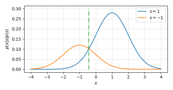
./image/basics_det_map_prop.png — Fig.34. Conditional probability of the transmitted signal $s$ given the received signal $x$.

Similarly if $p(s=-1)<p(s=1)$, the MAP decision boundary will look like

./image/basics_det_map_prop2.png — Fig.35. Conditional probability of the transmitted signal $s$ given the received signal $x$.

MAP looks more reasonable than ML, however, in practice, ML is widely used to detect/estimate the signal. One reason is that the signal from the transmitter is almost always randomized (or with scramble block), in other words roughly $p(s=1)=p(s=-1)=0.5$.

So far we discuss the detection of a constant signal from noise. How about detecting a waveform, instead of a constant, from noise? For example

$$ \begin{align} x[k] = s[k] + n[k]. \end{align} $$

At the receiver side, a correlation is conducted

$$ \begin{align} y &= \sum_{k=-\infty}^{\infty}{x[k]h[k]}\nonumber\\ &= \sum_{k=-\infty}^{\infty}{s[k]h[k]} + \sum_{k=-\infty}^{\infty}{n[k]h[k]}, \end{align} $$

where the first item is the signal, the second item is the noise, and $h[k]$ is the local reference signal. The goal here is to choose $h[k]$ to maximize the SNR (signal noise ratio), that is

$$ \begin{align} \mathop{\mathrm{argmax}}_{h[k]}{\frac{E((\sum_{k=-\infty}^{\infty}{s[k]h[k]})^2)}{E((\sum_{k=-\infty}^{\infty}{n[k]h[k]})^2)}}. \end{align} $$

The numerator can be simplified as

$$ \begin{align} E((\sum_{k=-\infty}^{\infty}{s[k]h[k]})^2) &= (\sum_{k=-\infty}^{\infty}{s[k]h[k]})^2\nonumber\\ &\leq \sum_{k=-\infty}^{\infty}{s[k]^2} \sum_{k=-\infty}^{\infty}{h[k]^2}, \end{align} $$

where the inequality comes from the Cauchy-Schwarz inequality. And two sides are equal if and only if $h[k]=c\cdot s[k]$, $\forall k$, where $c$ is a constant. The denominator can be simplified as

$$ \begin{align} E((\sum_{k=-\infty}^{\infty}{n[k]h[k]})^2) &= \sum_{k=-\infty}^{\infty}{E(n[k]^2)h[k]^2}\nonumber\\ &= \sigma^2\sum_{k=-\infty}^{\infty}{h[k]^2}, \end{align} $$

where $E(n[k]^2)=\sigma^2$. Here we assume $n[k]$ and $n[m]$ $\forall k\neq m$ are uncorrelated, that is $E(n[k]n[m])=0$. Thus

$$ \begin{align} \frac{E((\sum_{k=-\infty}^{\infty}{s[k]h[k]})^2)}{E((\sum_{k=-\infty}^{\infty}{n[k]h[k]})^2)} &\leq \frac{\sum_{k=-\infty}^{\infty}{s[k]^2}\sum_{k=-\infty}^{\infty}{h[k]^2}}{\sigma^2\sum_{k=-\infty}^{\infty}{h[k]^2}}\nonumber\\ &= \frac{\sum_{k=-\infty}^{\infty}{s[k]^2}}{\sigma^2}. \end{align} $$

The SNR achieve its maximum when $h[k]=c\cdot s[k]$, $\forall k$, where $c$ is constant (e.g., $c=1$). It is also called matched filter.

In OFDM, the original data is modulated to multiple orthogonal sub-carriers. ↩

Apply $x[n]$ to system $f_1$ first, then apply the output from $f_1$ to $f_2$. ↩

We do not take the symmetric filter coefficients into consideration. The procedure for symmetric coefficients is very similar. ↩

The range for 8 bit integer is -128,127. Since there are 3 bits before the decimal point, its range is $[-128/2^5, 127/2^5]$ ↩

In this trivial example, all filter coefficient is positive. Thus, there is no need to save the sign. ↩

The filter has 14 coefficients, which requires additional 4 bits. ↩